Supervised | Unsupervised Learning : Detecting and Evaluating Anomalies in Categorical Data Under Supervised and Unsupervised Settings
- 1. Table of Contents
- 1.1 Data Background
- 1.2 Data Description
- 1.3 Data Quality Assessment
- 1.4 Data Preprocessing
- 1.5 Data Exploration
- 1.6 Model Hyperparameter Tuning and Evaluation Preparation
- 1.7 Model Development With Synthetic Ground Truth Labels
- 1.8 Model Development Without Ground Truth Labels
- 1.9 Consolidated Findings
- 2. Summary
- 3. References
1. Table of Contents 
This project explores various Outlier Detection techniques specifically tailored for datasets with purely categorical features, utilizing multiple tools and libraries available in Python. The analysis was carried out in two distinct experimental settings: a Supervised Setting where synthetic outlier ground truth labels are available, and an Unsupervised Setting where no labels are assumed. The methods applied in both settings span a diverse range of non-deep learning techniques, including classical statistical, distance-based, and pattern-based models including: Isolation Forest, Clustering-Based Local Outlier Factor (CBLOF), K-Nearest Neighbors (KNN) and Histogram-Based Outlier Score (HBOS). In the supervised setting, outlier detection methods were evaluated using traditional classification metrics such as the Area Under the Receiver Operating Characteristic Curve(AUROC), F1-Score, and Precision@N to assess their ability to distinguish true outliers from normal observations. In contrast, the unsupervised setting employed label-agnostic evaluation strategies, leveraging internal and score-based metrics such as Silhouette Score on Outlier Scores, Outlier Score Entropy and Score Variance. These were complemented by Principal Component Analysis (PCA) and Uniform Manifold Approximation and Projection (UMAP) Visualizations to assess the score separability and clustering quality across methods. This dual-framework approach allows for a comprehensive understanding of how each method performs under both label-available and label-free conditions, providing a rigorous basis for outlier detection in categorical data contexts. All results were consolidated in a Summary presented at the end of the document.
Outlier Detection in datasets composed exclusively of categorical variables poses unique challenges because most traditional techniques rely on notions like distance, density, or variance—concepts naturally defined in numerical spaces. In contrast, categorical data lacks inherent numeric relationships or ordering, making it non-trivial to apply distance-based or distribution-based methods directly. However, there are still structured and principled approaches to identify anomalies in such datasets. At its core, an outlier in categorical data is an observation that exhibits a rare or unexpected combination of attribute levels. While each individual variable may contain common categories, their joint configuration may be highly improbable, making the observation an outlier even if no single variable is unusual in isolation. The most basic yet powerful approach begins by examining frequency distributions by way of tallying the count of each unique record configuration and flagging those that occur rarely or not at all in the rest of the data as potential anomalies. To go a step further, one can estimate probabilities of individual variable levels and their joint probabilities across combinations of features. This idea underlies models where the joint likelihood of feature values is used as an outlier score. However, due to the curse of dimensionality — even with a moderate number of variables — the number of possible category combinations grows exponentially, making pure joint frequency estimation unreliable in high dimensions. This motivates the use of dimensionality reduction techniques which maps categorical data into a continuous latent space. In this lower-dimensional space, standard outlier detection techniques can be applied more reliably. In other cases, categorical variables are transformed using encoding schemes to enable the use of well-established numeric algorithms. For instance, one-hot encoding represents each level of a categorical variable as a binary vector, while ordinal encoding assigns arbitrary numeric values to categories. More advanced encodings like entity embeddings can preserve semantic similarity between categories learned via neural networks. Once encoded, various outlier detection methods can be applied, provided the encoding faithfully retains category relationships. An alternative family of methods relies on clustering to group similar categorical records. Outliers are identified either as records not belonging to any dense cluster, or as records that lie far from their cluster's central profile. Finally, rule-based outlier detection extract conditional patterns and flag records that violate these frequent rules. In conclusion, while outlier detection in categorical data is fundamentally different from numeric data due to the lack of inherent distances or ordering, a combination of probability modeling, encoding and transformation, rule learning, and clustering can be used to detect anomalies effectively. The choice of method depends on the structure of the data, the cardinality of features, and whether interpretability or predictive performance is prioritized.
Outlier Detection In Categorical Data With Ground Truth Labels becomes a supervised classification task. In this setting, the goal is not just to detect anomalies, but to train models that can predict outlier status reliably, based on known labeled examples. This scenario is relatively rare in real-world applications, but it allows for robust evaluation and algorithm benchmarking. To begin, each observation in the dataset is tagged as either an "inlier" or an "outlier". This label can be derived from domain expertise, human annotation, or synthetic injection of anomalies for experimental setups. The categorical features are then encoded using techniques such as one-hot, ordinal, or entity embeddings so that they can be processed by standard supervised learning models or outlier scoring algorithms. Outlier detection methods are then trained on these encoded features. Even though these methods are typically unsupervised, in this scenario, their outputs—namely, the anomaly scores — can be evaluated using the known labels. Evaluation metrics for this setting include: Precision@N (a variation of precision that is particularly useful in ranking problems like outlier detection for evaluating the top N most confident predictions rather than all predictions), F1-Score (harmonic mean of precision and recall for balancing both metrics, particularly useful when there's a tradeoff), AUROC (Area Under the Receiver Operating Characteristic Curve) (evaluates the model’s ability to distinguish between inliers and outliers across various thresholds, where a higher value indicates better separability). This setup allows for quantitative comparison of different models and hyperparameters. Because true outliers are known, models can be ranked, tuned, and selected with confidence.
Outlier Detection In Categorical Data Without Ground Truth Labels is a purely unsupervised learning task. This introduces significant challenges: since the true identity of outliers is unknown, models cannot be trained or validated using standard supervised metrics. Instead, evaluation shifts toward the intrinsic structure of the data and the behavior of anomaly scores. To begin, categorical data must be carefully encoded using strategies that retain their semantic meaning. Common encoding methods include one-hot encoding (to preserve disjoint category identity), ordinal encoding (for ordered categories), and entity embeddings (to capture latent similarity among categories). Once the data is numerically represented, various unsupervised algorithms can be applied to compute outlier scores. These scores reflect the degree of "outlierness" of each observation based on algorithm-specific logic such as isolation depth, density deviation, or cluster distance. In the absence of ground truth labels, the quality of these scores is evaluated using unsupervised score-based metrics. These metrics help assess whether the algorithm has meaningfully differentiated outliers from inliers in a data-driven way including Outlier Score Entropy (measures the unpredictability or uniformity in the distribution of outlier scores where a very low entropy may indicate that the model is not distinguishing between normal and anomalous observations), score variance (examines the spread of anomaly scores across all observations where a low variance suggests that the model assigns similar scores to most points, possibly indicating insensitivity to actual structure), silhouette score on outlier scores (clusters the outlier scores themselves into two or more groups and evaluates how well-separated these clusters are with a high silhouette score suggesting that the model produces score groupings that align with distinguishable data behavior, reinforcing the meaningfulness of its outlier assignments) and clustering stability (assesses how consistent the outlier groupings remain when the input data or model parameters are slightly perturbed with low variability across runs implying that the model is robust and not overly sensitive to sampling artifacts, which boosts confidence in the flagged anomalies). These unsupervised evaluation techniques offer a practical lens through which model performance can be judged, even in the complete absence of labeled anomalies. When multiple models consistently flag the same observations as anomalous, or when scores exhibit structured and stable separation, this further validates the relevance of the identified outliers. Ultimately, there is no single "correct" model in unsupervised outlier detection without ground truth. Instead, a combination of score distribution analysis, clustering behavior, consistency checks, and domain interpretability is used to triangulate the credibility of the results. This makes practitioner insight and a deep understanding of the domain especially important when applying these methods to categorical data.
1.1. Data Background 
An open Thyroid Disease Dataset from Kaggle (with all credits attributed to Jai Naru and Abuchi Onwuegbusi) was used for the analysis as consolidated from the following primary sources:
- Reference Repository entitled Differentiated Thyroid Cancer Recurrence from UC Irvine Machine Learning Repository
- Research Paper entitled Machine Learning for Risk Stratification of Thyroid Cancer Patients: a 15-year Cohort Study from the European Archives of Oto-Rhino-Laryngology
This study hypothesized that the various clinicopathological characteristics influence differentiated thyroid cancer recurrence between patients.
The dichotomous categorical variable for the study is:
- Recurred - Status of the patient (Yes, Recurrence of differentiated thyroid cancer | No, No recurrence of differentiated thyroid cancer)
The predictor variables for the study are:
- Age - Patient's age (Years)
- Gender - Patient's sex (M | F)
- Smoking - Indication of smoking (Yes | No)
- Hx Smoking - Indication of smoking history (Yes | No)
- Hx Radiotherapy - Indication of radiotherapy history for any condition (Yes | No)
- Thyroid Function - Status of thyroid function (Clinical Hyperthyroidism, Hypothyroidism | Subclinical Hyperthyroidism, Hypothyroidism | Euthyroid)
- Physical Examination - Findings from physical examination including palpation of the thyroid gland and surrounding structures (Normal | Diffuse Goiter | Multinodular Goiter | Single Nodular Goiter Left, Right)
- Adenopathy - Indication of enlarged lymph nodes in the neck region (No | Right | Extensive | Left | Bilateral | Posterior)
- Pathology - Specific thyroid cancer type as determined by pathology examination of biopsy samples (Follicular | Hurthel Cell | Micropapillary | Papillary)
- Focality - Indication if the cancer is limited to one location or present in multiple locations (Uni-Focal | Multi-Focal)
- Risk - Risk category of the cancer based on various factors, such as tumor size, extent of spread, and histological type (Low | Intermediate | High)
- T - Tumor classification based on its size and extent of invasion into nearby structures (T1a | T1b | T2 | T3a | T3b | T4a | T4b)
- N - Nodal classification indicating the involvement of lymph nodes (N0 | N1a | N1b)
- M - Metastasis classification indicating the presence or absence of distant metastases (M0 | M1)
- Stage - Overall stage of the cancer, typically determined by combining T, N, and M classifications (I | II | III | IVa | IVb)
- Response - Cancer's response to treatment (Biochemical Incomplete | Indeterminate | Excellent | Structural Incomplete)
While the original dataset was designed for a categorical classification task predicting thyroid cancer recurrence, this study repurposes it for an outlier detection framework. In this revised context, the original response variable will be excluded, and only a subset of predictors—specifically those capturing clinicopathological characteristics—will be retained. These predictors will be converted into binary categorical variables to standardize representation. A synthetic binary response variable will then be generated using a frequency-based tagging strategy, labeling rare combinations of category levels as outliers and the rest as inliers. The goal is to estimate outlier scores for each observation and assess model performance in both supervised settings (using the synthetic labels) and unsupervised settings (without labels). This approach allows for evaluating the effectiveness of categorical outlier detection methods in a medically relevant context where rare clinicopathological profiles may signify atypical or high-risk cases.
1.2. Data Description 
- The initial tabular dataset was comprised of 383 observations and 17 variables (including 1 target and 16 predictors).
- 383 rows (observations)
- 17 columns (variables)
- 1/17 target (categorical)
- Recurred
- 1/17 predictor (numeric)
- Age
- 16/17 predictor (categorical)
- Gender
- Smoking
- Hx_Smoking
- Hx_Radiotherapy
- Thyroid_Function
- Physical_Examination
- Adenopathy
- Pathology
- Focality
- Risk
- T
- N
- M
- Stage
- Response
- 1/17 target (categorical)
##################################
# Loading Python Libraries
##################################
import numpy as np
import pandas as pd
import seaborn as sns
import matplotlib.pyplot as plt
import joblib
import itertools
import os
import pickle
import plotly.express as px
import plotly.io as pio
pio.renderers.default = 'notebook_connected'
%matplotlib inline

from operator import truediv
from sklearn.preprocessing import LabelEncoder
from scipy.stats import chi2_contingency, entropy

from sklearn.cluster import KMeans
from sklearn.decomposition import PCA
from sklearn.manifold import TSNE
from sklearn.metrics import silhouette_score, roc_auc_score, precision_score, f1_score
from sklearn.model_selection import train_test_split, StratifiedShuffleSplit, ParameterGrid
import umap.umap_ as umap

from pyod.models.knn import KNN
from pyod.models.hbos import HBOS
from pyod.models.cblof import CBLOF
from pyod.models.iforest import IForest

import warnings
warnings.filterwarnings("ignore", category=FutureWarning, module="sklearn")
warnings.filterwarnings("ignore", category=UserWarning, module="umap")
##################################
# Defining file paths
##################################
DATASETS_ORIGINAL_PATH = r"datasets\original"
DATASETS_FINAL_PATH = r"datasets\final\complete"
DATASETS_FINAL_TRAIN_PATH = r"datasets\final\train"
DATASETS_FINAL_TRAIN_FEATURES_PATH = r"datasets\final\train\features"
DATASETS_FINAL_TRAIN_TARGET_PATH = r"datasets\final\train\target"
DATASETS_FINAL_VALIDATION_PATH = r"datasets\final\validation"
DATASETS_FINAL_VALIDATION_FEATURES_PATH = r"datasets\final\validation\features"
DATASETS_FINAL_VALIDATION_TARGET_PATH = r"datasets\final\validation\target"
DATASETS_FINAL_TEST_PATH = r"datasets\final\test"
DATASETS_FINAL_TEST_FEATURES_PATH = r"datasets\final\test\features"
DATASETS_FINAL_TEST_TARGET_PATH = r"datasets\final\test\target"
MODELS_PATH = r"models"
##################################
# Loading the dataset
# from the DATASETS_ORIGINAL_PATH
##################################
thyroid_cancer = pd.read_csv(os.path.join("..", DATASETS_ORIGINAL_PATH, "Thyroid_Diff.csv"))
##################################
# Performing a general exploration of the dataset
##################################
print('Dataset Dimensions: ')
display(thyroid_cancer.shape)
Dataset Dimensions:
(383, 17)
##################################
# Listing the column names and data types
##################################
print('Column Names and Data Types:')
display(thyroid_cancer.dtypes)
Column Names and Data Types:
Age                      int64
Gender                  object
Smoking                 object
Hx Smoking              object
Hx Radiotherapy         object
Thyroid Function        object
Physical Examination    object
Adenopathy              object
Pathology               object
Focality                object
Risk                    object
T                       object
N                       object
M                       object
Stage                   object
Response                object
Recurred                object
dtype: object
##################################
# Renaming and standardizing the column names
# to replace blanks with undercores
##################################
thyroid_cancer.columns = thyroid_cancer.columns.str.replace(" ", "_")
##################################
# Taking a snapshot of the dataset
##################################
thyroid_cancer.head()
| Age | Gender | Smoking | Hx_Smoking | Hx_Radiotherapy | Thyroid_Function | Physical_Examination | Adenopathy | Pathology | Focality | Risk | T | N | M | Stage | Response | Recurred | |
|---|---|---|---|---|---|---|---|---|---|---|---|---|---|---|---|---|---|
| 0 | 27 | F | No | No | No | Euthyroid | Single nodular goiter-left | No | Micropapillary | Uni-Focal | Low | T1a | N0 | M0 | I | Indeterminate | No |
| 1 | 34 | F | No | Yes | No | Euthyroid | Multinodular goiter | No | Micropapillary | Uni-Focal | Low | T1a | N0 | M0 | I | Excellent | No |
| 2 | 30 | F | No | No | No | Euthyroid | Single nodular goiter-right | No | Micropapillary | Uni-Focal | Low | T1a | N0 | M0 | I | Excellent | No |
| 3 | 62 | F | No | No | No | Euthyroid | Single nodular goiter-right | No | Micropapillary | Uni-Focal | Low | T1a | N0 | M0 | I | Excellent | No |
| 4 | 62 | F | No | No | No | Euthyroid | Multinodular goiter | No | Micropapillary | Multi-Focal | Low | T1a | N0 | M0 | I | Excellent | No |
##################################
# Selecting categorical columns (both object and categorical types)
# and listing the unique categorical levels
##################################
cat_cols = thyroid_cancer.select_dtypes(include=["object", "category"]).columns
for col in cat_cols:
    print(f"Categorical | Object Column: {col}")
    print(thyroid_cancer[col].unique())
    print("-" * 40)
Categorical | Object Column: Gender
['F' 'M']
----------------------------------------
Categorical | Object Column: Smoking
['No' 'Yes']
----------------------------------------
Categorical | Object Column: Hx_Smoking
['No' 'Yes']
----------------------------------------
Categorical | Object Column: Hx_Radiotherapy
['No' 'Yes']
----------------------------------------
Categorical | Object Column: Thyroid_Function
['Euthyroid' 'Clinical Hyperthyroidism' 'Clinical Hypothyroidism'
 'Subclinical Hyperthyroidism' 'Subclinical Hypothyroidism']
----------------------------------------
Categorical | Object Column: Physical_Examination
['Single nodular goiter-left' 'Multinodular goiter'
 'Single nodular goiter-right' 'Normal' 'Diffuse goiter']
----------------------------------------
Categorical | Object Column: Adenopathy
['No' 'Right' 'Extensive' 'Left' 'Bilateral' 'Posterior']
----------------------------------------
Categorical | Object Column: Pathology
['Micropapillary' 'Papillary' 'Follicular' 'Hurthel cell']
----------------------------------------
Categorical | Object Column: Focality
['Uni-Focal' 'Multi-Focal']
----------------------------------------
Categorical | Object Column: Risk
['Low' 'Intermediate' 'High']
----------------------------------------
Categorical | Object Column: T
['T1a' 'T1b' 'T2' 'T3a' 'T3b' 'T4a' 'T4b']
----------------------------------------
Categorical | Object Column: N
['N0' 'N1b' 'N1a']
----------------------------------------
Categorical | Object Column: M
['M0' 'M1']
----------------------------------------
Categorical | Object Column: Stage
['I' 'II' 'IVB' 'III' 'IVA']
----------------------------------------
Categorical | Object Column: Response
['Indeterminate' 'Excellent' 'Structural Incomplete'
 'Biochemical Incomplete']
----------------------------------------
Categorical | Object Column: Recurred
['No' 'Yes']
----------------------------------------
##################################
# Correcting a category level
##################################
thyroid_cancer["Pathology"] = thyroid_cancer["Pathology"].replace("Hurthel cell", "Hurthle Cell")
##################################
# Setting the levels of the categorical variables
##################################
thyroid_cancer['Recurred'] = thyroid_cancer['Recurred'].astype('category')
thyroid_cancer['Recurred'] = thyroid_cancer['Recurred'].cat.set_categories(['No', 'Yes'], ordered=True)
thyroid_cancer['Gender'] = thyroid_cancer['Gender'].astype('category')
thyroid_cancer['Gender'] = thyroid_cancer['Gender'].cat.set_categories(['M', 'F'], ordered=True)
thyroid_cancer['Smoking'] = thyroid_cancer['Smoking'].astype('category')
thyroid_cancer['Smoking'] = thyroid_cancer['Smoking'].cat.set_categories(['No', 'Yes'], ordered=True)
thyroid_cancer['Hx_Smoking'] = thyroid_cancer['Hx_Smoking'].astype('category')
thyroid_cancer['Hx_Smoking'] = thyroid_cancer['Hx_Smoking'].cat.set_categories(['No', 'Yes'], ordered=True)
thyroid_cancer['Hx_Radiotherapy'] = thyroid_cancer['Hx_Radiotherapy'].astype('category')
thyroid_cancer['Hx_Radiotherapy'] = thyroid_cancer['Hx_Radiotherapy'].cat.set_categories(['No', 'Yes'], ordered=True)
thyroid_cancer['Thyroid_Function'] = thyroid_cancer['Thyroid_Function'].astype('category')
thyroid_cancer['Thyroid_Function'] = thyroid_cancer['Thyroid_Function'].cat.set_categories(['Euthyroid', 'Subclinical Hypothyroidism', 'Subclinical Hyperthyroidism', 'Clinical Hypothyroidism', 'Clinical Hyperthyroidism'], ordered=True)
thyroid_cancer['Physical_Examination'] = thyroid_cancer['Physical_Examination'].astype('category')
thyroid_cancer['Physical_Examination'] = thyroid_cancer['Physical_Examination'].cat.set_categories(['Normal', 'Single nodular goiter-left', 'Single nodular goiter-right', 'Multinodular goiter', 'Diffuse goiter'], ordered=True)
thyroid_cancer['Adenopathy'] = thyroid_cancer['Adenopathy'].astype('category')
thyroid_cancer['Adenopathy'] = thyroid_cancer['Adenopathy'].cat.set_categories(['No', 'Left', 'Right', 'Bilateral', 'Posterior', 'Extensive'], ordered=True)
thyroid_cancer['Pathology'] = thyroid_cancer['Pathology'].astype('category')
thyroid_cancer['Pathology'] = thyroid_cancer['Pathology'].cat.set_categories(['Hurthle Cell', 'Follicular', 'Micropapillary', 'Papillary'], ordered=True)
thyroid_cancer['Focality'] = thyroid_cancer['Focality'].astype('category')
thyroid_cancer['Focality'] = thyroid_cancer['Focality'].cat.set_categories(['Uni-Focal', 'Multi-Focal'], ordered=True)
thyroid_cancer['Risk'] = thyroid_cancer['Risk'].astype('category')
thyroid_cancer['Risk'] = thyroid_cancer['Risk'].cat.set_categories(['Low', 'Intermediate', 'High'], ordered=True)
thyroid_cancer['T'] = thyroid_cancer['T'].astype('category')
thyroid_cancer['T'] = thyroid_cancer['T'].cat.set_categories(['T1a', 'T1b', 'T2', 'T3a', 'T3b', 'T4a', 'T4b'], ordered=True)
thyroid_cancer['N'] = thyroid_cancer['N'].astype('category')
thyroid_cancer['N'] = thyroid_cancer['N'].cat.set_categories(['N0', 'N1a', 'N1b'], ordered=True)
thyroid_cancer['M'] = thyroid_cancer['M'].astype('category')
thyroid_cancer['M'] = thyroid_cancer['M'].cat.set_categories(['M0', 'M1'], ordered=True)
thyroid_cancer['Stage'] = thyroid_cancer['Stage'].astype('category')
thyroid_cancer['Stage'] = thyroid_cancer['Stage'].cat.set_categories(['I', 'II', 'III', 'IVA', 'IVB'], ordered=True)
thyroid_cancer['Response'] = thyroid_cancer['Response'].astype('category')
thyroid_cancer['Response'] = thyroid_cancer['Response'].cat.set_categories(['Excellent', 'Structural Incomplete', 'Biochemical Incomplete', 'Indeterminate'], ordered=True)
##################################
# Performing a general exploration of the numeric variables
##################################
print('Numeric Variable Summary:')
display(thyroid_cancer.describe(include='number').transpose())
Numeric Variable Summary:
| count | mean | std | min | 25% | 50% | 75% | max | |
|---|---|---|---|---|---|---|---|---|
| Age | 383.0 | 40.866841 | 15.134494 | 15.0 | 29.0 | 37.0 | 51.0 | 82.0 |
##################################
# Performing a general exploration of the categorical variables
##################################
print('Categorical Variable Summary:')
display(thyroid_cancer.describe(include='category').transpose())
Categorical Variable Summary:
| count | unique | top | freq | |
|---|---|---|---|---|
| Gender | 383 | 2 | F | 312 |
| Smoking | 383 | 2 | No | 334 |
| Hx_Smoking | 383 | 2 | No | 355 |
| Hx_Radiotherapy | 383 | 2 | No | 376 |
| Thyroid_Function | 383 | 5 | Euthyroid | 332 |
| Physical_Examination | 383 | 5 | Single nodular goiter-right | 140 |
| Adenopathy | 383 | 6 | No | 277 |
| Pathology | 383 | 4 | Papillary | 287 |
| Focality | 383 | 2 | Uni-Focal | 247 |
| Risk | 383 | 3 | Low | 249 |
| T | 383 | 7 | T2 | 151 |
| N | 383 | 3 | N0 | 268 |
| M | 383 | 2 | M0 | 365 |
| Stage | 383 | 5 | I | 333 |
| Response | 383 | 4 | Excellent | 208 |
| Recurred | 383 | 2 | No | 275 |
##################################
# Performing a general exploration of the categorical variable levels
# based on the ordered categories
##################################
ordered_cat_cols = thyroid_cancer.select_dtypes(include=["category"]).columns
for col in ordered_cat_cols:
    print(f"Column: {col}")
    print("Absolute Frequencies:")
    print(thyroid_cancer[col].value_counts().reindex(thyroid_cancer[col].cat.categories))
    print("\nNormalized Frequencies:")
    print(thyroid_cancer[col].value_counts(normalize=True).reindex(thyroid_cancer[col].cat.categories))
    print("-" * 50)
Column: Gender
Absolute Frequencies:
M     71
F    312
Name: count, dtype: int64

Normalized Frequencies:
M    0.185379
F    0.814621
Name: proportion, dtype: float64
--------------------------------------------------
Column: Smoking
Absolute Frequencies:
No     334
Yes     49
Name: count, dtype: int64

Normalized Frequencies:
No     0.872063
Yes    0.127937
Name: proportion, dtype: float64
--------------------------------------------------
Column: Hx_Smoking
Absolute Frequencies:
No     355
Yes     28
Name: count, dtype: int64

Normalized Frequencies:
No     0.926893
Yes    0.073107
Name: proportion, dtype: float64
--------------------------------------------------
Column: Hx_Radiotherapy
Absolute Frequencies:
No     376
Yes      7
Name: count, dtype: int64

Normalized Frequencies:
No     0.981723
Yes    0.018277
Name: proportion, dtype: float64
--------------------------------------------------
Column: Thyroid_Function
Absolute Frequencies:
Euthyroid                      332
Subclinical Hypothyroidism      14
Subclinical Hyperthyroidism      5
Clinical Hypothyroidism         12
Clinical Hyperthyroidism        20
Name: count, dtype: int64

Normalized Frequencies:
Euthyroid                      0.866841
Subclinical Hypothyroidism     0.036554
Subclinical Hyperthyroidism    0.013055
Clinical Hypothyroidism        0.031332
Clinical Hyperthyroidism       0.052219
Name: proportion, dtype: float64
--------------------------------------------------
Column: Physical_Examination
Absolute Frequencies:
Normal                           7
Single nodular goiter-left      89
Single nodular goiter-right    140
Multinodular goiter            140
Diffuse goiter                   7
Name: count, dtype: int64

Normalized Frequencies:
Normal                         0.018277
Single nodular goiter-left     0.232376
Single nodular goiter-right    0.365535
Multinodular goiter            0.365535
Diffuse goiter                 0.018277
Name: proportion, dtype: float64
--------------------------------------------------
Column: Adenopathy
Absolute Frequencies:
No           277
Left          17
Right         48
Bilateral     32
Posterior      2
Extensive      7
Name: count, dtype: int64

Normalized Frequencies:
No           0.723238
Left         0.044386
Right        0.125326
Bilateral    0.083551
Posterior    0.005222
Extensive    0.018277
Name: proportion, dtype: float64
--------------------------------------------------
Column: Pathology
Absolute Frequencies:
Hurthle Cell       20
Follicular         28
Micropapillary     48
Papillary         287
Name: count, dtype: int64

Normalized Frequencies:
Hurthle Cell      0.052219
Follicular        0.073107
Micropapillary    0.125326
Papillary         0.749347
Name: proportion, dtype: float64
--------------------------------------------------
Column: Focality
Absolute Frequencies:
Uni-Focal      247
Multi-Focal    136
Name: count, dtype: int64

Normalized Frequencies:
Uni-Focal      0.644909
Multi-Focal    0.355091
Name: proportion, dtype: float64
--------------------------------------------------
Column: Risk
Absolute Frequencies:
Low             249
Intermediate    102
High             32
Name: count, dtype: int64

Normalized Frequencies:
Low             0.650131
Intermediate    0.266319
High            0.083551
Name: proportion, dtype: float64
--------------------------------------------------
Column: T
Absolute Frequencies:
T1a     49
T1b     43
T2     151
T3a     96
T3b     16
T4a     20
T4b      8
Name: count, dtype: int64

Normalized Frequencies:
T1a    0.127937
T1b    0.112272
T2     0.394256
T3a    0.250653
T3b    0.041775
T4a    0.052219
T4b    0.020888
Name: proportion, dtype: float64
--------------------------------------------------
Column: N
Absolute Frequencies:
N0     268
N1a     22
N1b     93
Name: count, dtype: int64

Normalized Frequencies:
N0     0.699739
N1a    0.057441
N1b    0.242820
Name: proportion, dtype: float64
--------------------------------------------------
Column: M
Absolute Frequencies:
M0    365
M1     18
Name: count, dtype: int64

Normalized Frequencies:
M0    0.953003
M1    0.046997
Name: proportion, dtype: float64
--------------------------------------------------
Column: Stage
Absolute Frequencies:
I      333
II      32
III      4
IVA      3
IVB     11
Name: count, dtype: int64

Normalized Frequencies:
I      0.869452
II     0.083551
III    0.010444
IVA    0.007833
IVB    0.028721
Name: proportion, dtype: float64
--------------------------------------------------
Column: Response
Absolute Frequencies:
Excellent                 208
Structural Incomplete      91
Biochemical Incomplete     23
Indeterminate              61
Name: count, dtype: int64

Normalized Frequencies:
Excellent                 0.543081
Structural Incomplete     0.237598
Biochemical Incomplete    0.060052
Indeterminate             0.159269
Name: proportion, dtype: float64
--------------------------------------------------
Column: Recurred
Absolute Frequencies:
No     275
Yes    108
Name: count, dtype: int64

Normalized Frequencies:
No     0.718016
Yes    0.281984
Name: proportion, dtype: float64
--------------------------------------------------
1.3. Data Quality Assessment 
Data quality findings based on assessment are as follows:
- A total of 19 duplicated rows were identified.
- In total, 34 observations were affected, consisting of 16 unique occurrences and 19 subsequent duplicates.
- These 19 duplicates spanned 16 distinct variations, meaning some variations had multiple duplicates.
- To clean the dataset, all 19 duplicate rows were removed, retaining only the first occurrence of each of the 16 unique variations.
- No missing data noted for any variable with Null.Count>0 and Fill.Rate<1.0.
- Low variance observed for 8 variables with First.Second.Mode.Ratio>5.
- Hx_Radiotherapy: First.Second.Mode.Ratio = 51.000 (comprised 2 category levels)
- M: First.Second.Mode.Ratio = 19.222 (comprised 2 category levels)
- Thyroid_Function: First.Second.Mode.Ratio = 15.650 (comprised 5 category levels)
- Hx_Smoking: First.Second.Mode.Ratio = 12.000 (comprised 2 category levels)
- Stage: First.Second.Mode.Ratio = 9.812 (comprised 5 category levels)
- Smoking: First.Second.Mode.Ratio = 6.428 (comprised 2 category levels)
- Pathology: First.Second.Mode.Ratio = 6.022 (comprised 4 category levels)
- Adenopathy: First.Second.Mode.Ratio = 5.375 (comprised 5 category levels)
- No low variance observed for any variable with Unique.Count.Ratio>10.
- No high skewness observed for any variable with Skewness>3 or Skewness<(-3).
##################################
# Counting the number of duplicated rows
##################################
thyroid_cancer.duplicated().sum()
np.int64(19)
##################################
# Exploring the duplicated rows
##################################
duplicated_rows = thyroid_cancer[thyroid_cancer.duplicated(keep=False)]
display(duplicated_rows)
| Age | Gender | Smoking | Hx_Smoking | Hx_Radiotherapy | Thyroid_Function | Physical_Examination | Adenopathy | Pathology | Focality | Risk | T | N | M | Stage | Response | Recurred | |
|---|---|---|---|---|---|---|---|---|---|---|---|---|---|---|---|---|---|
| 8 | 51 | F | No | No | No | Euthyroid | Single nodular goiter-right | No | Micropapillary | Uni-Focal | Low | T1a | N0 | M0 | I | Excellent | No |
| 9 | 40 | F | No | No | No | Euthyroid | Single nodular goiter-right | No | Micropapillary | Uni-Focal | Low | T1a | N0 | M0 | I | Excellent | No |
| 22 | 36 | F | No | No | No | Euthyroid | Single nodular goiter-right | No | Micropapillary | Uni-Focal | Low | T1a | N0 | M0 | I | Excellent | No |
| 32 | 36 | F | No | No | No | Euthyroid | Single nodular goiter-right | No | Micropapillary | Uni-Focal | Low | T1a | N0 | M0 | I | Excellent | No |
| 38 | 40 | F | No | No | No | Euthyroid | Single nodular goiter-right | No | Micropapillary | Uni-Focal | Low | T1a | N0 | M0 | I | Excellent | No |
| 40 | 51 | F | No | No | No | Euthyroid | Single nodular goiter-right | No | Micropapillary | Uni-Focal | Low | T1a | N0 | M0 | I | Excellent | No |
| 61 | 35 | F | No | No | No | Euthyroid | Single nodular goiter-right | No | Papillary | Uni-Focal | Low | T1b | N0 | M0 | I | Excellent | No |
| 66 | 35 | F | No | No | No | Euthyroid | Single nodular goiter-right | No | Papillary | Uni-Focal | Low | T1b | N0 | M0 | I | Excellent | No |
| 67 | 51 | F | No | No | No | Euthyroid | Single nodular goiter-left | No | Papillary | Uni-Focal | Low | T1b | N0 | M0 | I | Excellent | No |
| 69 | 51 | F | No | No | No | Euthyroid | Single nodular goiter-left | No | Papillary | Uni-Focal | Low | T1b | N0 | M0 | I | Excellent | No |
| 73 | 29 | F | No | No | No | Euthyroid | Single nodular goiter-right | No | Papillary | Uni-Focal | Low | T1b | N0 | M0 | I | Excellent | No |
| 77 | 29 | F | No | No | No | Euthyroid | Single nodular goiter-right | No | Papillary | Uni-Focal | Low | T1b | N0 | M0 | I | Excellent | No |
| 106 | 26 | F | No | No | No | Euthyroid | Multinodular goiter | No | Papillary | Uni-Focal | Low | T2 | N0 | M0 | I | Excellent | No |
| 110 | 31 | F | No | No | No | Euthyroid | Single nodular goiter-right | No | Papillary | Uni-Focal | Low | T2 | N0 | M0 | I | Excellent | No |
| 113 | 32 | F | No | No | No | Euthyroid | Single nodular goiter-right | No | Papillary | Uni-Focal | Low | T2 | N0 | M0 | I | Excellent | No |
| 115 | 37 | F | No | No | No | Euthyroid | Single nodular goiter-right | No | Papillary | Uni-Focal | Low | T2 | N0 | M0 | I | Excellent | No |
| 119 | 28 | F | No | No | No | Euthyroid | Single nodular goiter-right | No | Papillary | Uni-Focal | Low | T2 | N0 | M0 | I | Excellent | No |
| 120 | 37 | F | No | No | No | Euthyroid | Single nodular goiter-right | No | Papillary | Uni-Focal | Low | T2 | N0 | M0 | I | Excellent | No |
| 121 | 26 | F | No | No | No | Euthyroid | Multinodular goiter | No | Papillary | Uni-Focal | Low | T2 | N0 | M0 | I | Excellent | No |
| 123 | 28 | F | No | No | No | Euthyroid | Single nodular goiter-right | No | Papillary | Uni-Focal | Low | T2 | N0 | M0 | I | Excellent | No |
| 132 | 32 | F | No | No | No | Euthyroid | Single nodular goiter-right | No | Papillary | Uni-Focal | Low | T2 | N0 | M0 | I | Excellent | No |
| 136 | 21 | F | No | No | No | Euthyroid | Single nodular goiter-right | No | Papillary | Uni-Focal | Low | T2 | N0 | M0 | I | Excellent | No |
| 137 | 32 | F | No | No | No | Euthyroid | Single nodular goiter-right | No | Papillary | Uni-Focal | Low | T2 | N0 | M0 | I | Excellent | No |
| 138 | 26 | F | No | No | No | Euthyroid | Multinodular goiter | No | Papillary | Uni-Focal | Low | T2 | N0 | M0 | I | Excellent | No |
| 142 | 42 | F | No | No | No | Euthyroid | Multinodular goiter | No | Papillary | Uni-Focal | Low | T2 | N0 | M0 | I | Excellent | No |
| 161 | 22 | F | No | No | No | Euthyroid | Single nodular goiter-right | No | Papillary | Uni-Focal | Low | T2 | N0 | M0 | I | Excellent | No |
| 166 | 31 | F | No | No | No | Euthyroid | Single nodular goiter-right | No | Papillary | Uni-Focal | Low | T2 | N0 | M0 | I | Excellent | No |
| 168 | 21 | F | No | No | No | Euthyroid | Single nodular goiter-right | No | Papillary | Uni-Focal | Low | T2 | N0 | M0 | I | Excellent | No |
| 170 | 38 | F | No | No | No | Euthyroid | Single nodular goiter-right | No | Papillary | Uni-Focal | Low | T2 | N0 | M0 | I | Excellent | No |
| 175 | 34 | F | No | No | No | Euthyroid | Multinodular goiter | No | Papillary | Uni-Focal | Low | T2 | N0 | M0 | I | Excellent | No |
| 178 | 38 | F | No | No | No | Euthyroid | Single nodular goiter-right | No | Papillary | Uni-Focal | Low | T2 | N0 | M0 | I | Excellent | No |
| 183 | 26 | F | No | No | No | Euthyroid | Multinodular goiter | No | Papillary | Uni-Focal | Low | T2 | N0 | M0 | I | Excellent | No |
| 187 | 34 | F | No | No | No | Euthyroid | Multinodular goiter | No | Papillary | Uni-Focal | Low | T2 | N0 | M0 | I | Excellent | No |
| 189 | 42 | F | No | No | No | Euthyroid | Multinodular goiter | No | Papillary | Uni-Focal | Low | T2 | N0 | M0 | I | Excellent | No |
| 196 | 22 | F | No | No | No | Euthyroid | Single nodular goiter-right | No | Papillary | Uni-Focal | Low | T2 | N0 | M0 | I | Excellent | No |
##################################
# Checking if duplicated rows have identical values across all columns
##################################
num_unique_dup_rows = duplicated_rows.drop_duplicates().shape[0]
num_total_dup_rows = duplicated_rows.shape[0]
if num_unique_dup_rows == 1:
    print("All duplicated rows have the same values across all columns.")
else:
    print(f"There are {num_unique_dup_rows} unique versions among the {num_total_dup_rows} duplicated rows.")
There are 16 unique versions among the 35 duplicated rows.
##################################
# Counting the unique variations among duplicated rows
##################################
unique_dup_variations = duplicated_rows.drop_duplicates()
variation_counts = duplicated_rows.value_counts().reset_index(name="Count")
print("Unique duplicated row variations and their counts:")
display(variation_counts)
Unique duplicated row variations and their counts:
| Age | Gender | Smoking | Hx_Smoking | Hx_Radiotherapy | Thyroid_Function | Physical_Examination | Adenopathy | Pathology | Focality | Risk | T | N | M | Stage | Response | Recurred | Count | |
|---|---|---|---|---|---|---|---|---|---|---|---|---|---|---|---|---|---|---|
| 0 | 26 | F | No | No | No | Euthyroid | Multinodular goiter | No | Papillary | Uni-Focal | Low | T2 | N0 | M0 | I | Excellent | No | 4 |
| 1 | 32 | F | No | No | No | Euthyroid | Single nodular goiter-right | No | Papillary | Uni-Focal | Low | T2 | N0 | M0 | I | Excellent | No | 3 |
| 2 | 22 | F | No | No | No | Euthyroid | Single nodular goiter-right | No | Papillary | Uni-Focal | Low | T2 | N0 | M0 | I | Excellent | No | 2 |
| 3 | 21 | F | No | No | No | Euthyroid | Single nodular goiter-right | No | Papillary | Uni-Focal | Low | T2 | N0 | M0 | I | Excellent | No | 2 |
| 4 | 28 | F | No | No | No | Euthyroid | Single nodular goiter-right | No | Papillary | Uni-Focal | Low | T2 | N0 | M0 | I | Excellent | No | 2 |
| 5 | 29 | F | No | No | No | Euthyroid | Single nodular goiter-right | No | Papillary | Uni-Focal | Low | T1b | N0 | M0 | I | Excellent | No | 2 |
| 6 | 31 | F | No | No | No | Euthyroid | Single nodular goiter-right | No | Papillary | Uni-Focal | Low | T2 | N0 | M0 | I | Excellent | No | 2 |
| 7 | 34 | F | No | No | No | Euthyroid | Multinodular goiter | No | Papillary | Uni-Focal | Low | T2 | N0 | M0 | I | Excellent | No | 2 |
| 8 | 35 | F | No | No | No | Euthyroid | Single nodular goiter-right | No | Papillary | Uni-Focal | Low | T1b | N0 | M0 | I | Excellent | No | 2 |
| 9 | 36 | F | No | No | No | Euthyroid | Single nodular goiter-right | No | Micropapillary | Uni-Focal | Low | T1a | N0 | M0 | I | Excellent | No | 2 |
| 10 | 37 | F | No | No | No | Euthyroid | Single nodular goiter-right | No | Papillary | Uni-Focal | Low | T2 | N0 | M0 | I | Excellent | No | 2 |
| 11 | 38 | F | No | No | No | Euthyroid | Single nodular goiter-right | No | Papillary | Uni-Focal | Low | T2 | N0 | M0 | I | Excellent | No | 2 |
| 12 | 40 | F | No | No | No | Euthyroid | Single nodular goiter-right | No | Micropapillary | Uni-Focal | Low | T1a | N0 | M0 | I | Excellent | No | 2 |
| 13 | 42 | F | No | No | No | Euthyroid | Multinodular goiter | No | Papillary | Uni-Focal | Low | T2 | N0 | M0 | I | Excellent | No | 2 |
| 14 | 51 | F | No | No | No | Euthyroid | Single nodular goiter-left | No | Papillary | Uni-Focal | Low | T1b | N0 | M0 | I | Excellent | No | 2 |
| 15 | 51 | F | No | No | No | Euthyroid | Single nodular goiter-right | No | Micropapillary | Uni-Focal | Low | T1a | N0 | M0 | I | Excellent | No | 2 |
##################################
# Removing the duplicated rows and
# retaining only the first occurrence
##################################
thyroid_cancer_row_filtered = thyroid_cancer.drop_duplicates(keep="first")
print('Dataset Dimensions: ')
display(thyroid_cancer_row_filtered.shape)
Dataset Dimensions:
(364, 17)
##################################
# Gathering the data types for each column
##################################
data_type_list = list(thyroid_cancer_row_filtered.dtypes)
##################################
# Gathering the variable names for each column
##################################
variable_name_list = list(thyroid_cancer_row_filtered.columns)
##################################
# Gathering the number of observations for each column
##################################
row_count_list = list([len(thyroid_cancer_row_filtered)] * len(thyroid_cancer_row_filtered.columns))
##################################
# Gathering the number of missing data for each column
##################################
null_count_list = list(thyroid_cancer_row_filtered.isna().sum(axis=0))
##################################
# Gathering the number of non-missing data for each column
##################################
non_null_count_list = list(thyroid_cancer_row_filtered.count())
##################################
# Gathering the missing data percentage for each column
##################################
fill_rate_list = map(truediv, non_null_count_list, row_count_list)
##################################
# Formulating the summary
# for all columns
##################################
all_column_quality_summary = pd.DataFrame(zip(variable_name_list,
                                              data_type_list,
                                              row_count_list,
                                              non_null_count_list,
                                              null_count_list,
                                              fill_rate_list),
                                        columns=['Column.Name',
                                                 'Column.Type',
                                                 'Row.Count',
                                                 'Non.Null.Count',
                                                 'Null.Count',
                                                 'Fill.Rate'])
display(all_column_quality_summary)
| Column.Name | Column.Type | Row.Count | Non.Null.Count | Null.Count | Fill.Rate | |
|---|---|---|---|---|---|---|
| 0 | Age | int64 | 364 | 364 | 0 | 1.0 |
| 1 | Gender | category | 364 | 364 | 0 | 1.0 |
| 2 | Smoking | category | 364 | 364 | 0 | 1.0 |
| 3 | Hx_Smoking | category | 364 | 364 | 0 | 1.0 |
| 4 | Hx_Radiotherapy | category | 364 | 364 | 0 | 1.0 |
| 5 | Thyroid_Function | category | 364 | 364 | 0 | 1.0 |
| 6 | Physical_Examination | category | 364 | 364 | 0 | 1.0 |
| 7 | Adenopathy | category | 364 | 364 | 0 | 1.0 |
| 8 | Pathology | category | 364 | 364 | 0 | 1.0 |
| 9 | Focality | category | 364 | 364 | 0 | 1.0 |
| 10 | Risk | category | 364 | 364 | 0 | 1.0 |
| 11 | T | category | 364 | 364 | 0 | 1.0 |
| 12 | N | category | 364 | 364 | 0 | 1.0 |
| 13 | M | category | 364 | 364 | 0 | 1.0 |
| 14 | Stage | category | 364 | 364 | 0 | 1.0 |
| 15 | Response | category | 364 | 364 | 0 | 1.0 |
| 16 | Recurred | category | 364 | 364 | 0 | 1.0 |
##################################
# Counting the number of columns
# with Fill.Rate < 1.00
##################################
len(all_column_quality_summary[(all_column_quality_summary['Fill.Rate']<1)])
0
##################################
# Identifying the rows
# with Fill.Rate < 0.90
##################################
column_low_fill_rate = all_column_quality_summary[(all_column_quality_summary['Fill.Rate']<0.90)]
##################################
# Gathering the indices for each observation
##################################
row_index_list = thyroid_cancer_row_filtered.index
##################################
# Gathering the number of columns for each observation
##################################
column_count_list = list([len(thyroid_cancer_row_filtered.columns)] * len(thyroid_cancer_row_filtered))
##################################
# Gathering the number of missing data for each row
##################################
null_row_list = list(thyroid_cancer_row_filtered.isna().sum(axis=1))
##################################
# Gathering the missing data percentage for each column
##################################
missing_rate_list = map(truediv, null_row_list, column_count_list)
##################################
# Identifying the rows
# with missing data
##################################
all_row_quality_summary = pd.DataFrame(zip(row_index_list,
                                           column_count_list,
                                           null_row_list,
                                           missing_rate_list),
                                        columns=['Row.Name',
                                                 'Column.Count',
                                                 'Null.Count',
                                                 'Missing.Rate'])
display(all_row_quality_summary)
| Row.Name | Column.Count | Null.Count | Missing.Rate | |
|---|---|---|---|---|
| 0 | 0 | 17 | 0 | 0.0 |
| 1 | 1 | 17 | 0 | 0.0 |
| 2 | 2 | 17 | 0 | 0.0 |
| 3 | 3 | 17 | 0 | 0.0 |
| 4 | 4 | 17 | 0 | 0.0 |
| ... | ... | ... | ... | ... |
| 359 | 378 | 17 | 0 | 0.0 |
| 360 | 379 | 17 | 0 | 0.0 |
| 361 | 380 | 17 | 0 | 0.0 |
| 362 | 381 | 17 | 0 | 0.0 |
| 363 | 382 | 17 | 0 | 0.0 |
364 rows × 4 columns
##################################
# Counting the number of rows
# with Missing.Rate > 0.00
##################################
len(all_row_quality_summary[(all_row_quality_summary['Missing.Rate']>0.00)])
0
##################################
# Formulating the dataset
# with numeric columns only
##################################
thyroid_cancer_numeric = thyroid_cancer_row_filtered.select_dtypes(include='number')
##################################
# Gathering the variable names for each numeric column
##################################
numeric_variable_name_list = thyroid_cancer_numeric.columns
##################################
# Gathering the minimum value for each numeric column
##################################
numeric_minimum_list = thyroid_cancer_numeric.min()
##################################
# Gathering the mean value for each numeric column
##################################
numeric_mean_list = thyroid_cancer_numeric.mean()
##################################
# Gathering the median value for each numeric column
##################################
numeric_median_list = thyroid_cancer_numeric.median()
##################################
# Gathering the maximum value for each numeric column
##################################
numeric_maximum_list = thyroid_cancer_numeric.max()
##################################
# Gathering the first mode values for each numeric column
##################################
numeric_first_mode_list = [thyroid_cancer_row_filtered[x].value_counts(dropna=True).index.tolist()[0] for x in thyroid_cancer_numeric]
##################################
# Gathering the second mode values for each numeric column
##################################
numeric_second_mode_list = [thyroid_cancer_row_filtered[x].value_counts(dropna=True).index.tolist()[1] for x in thyroid_cancer_numeric]
##################################
# Gathering the count of first mode values for each numeric column
##################################
numeric_first_mode_count_list = [thyroid_cancer_numeric[x].isin([thyroid_cancer_row_filtered[x].value_counts(dropna=True).index.tolist()[0]]).sum() for x in thyroid_cancer_numeric]
##################################
# Gathering the count of second mode values for each numeric column
##################################
numeric_second_mode_count_list = [thyroid_cancer_numeric[x].isin([thyroid_cancer_row_filtered[x].value_counts(dropna=True).index.tolist()[1]]).sum() for x in thyroid_cancer_numeric]
##################################
# Gathering the first mode to second mode ratio for each numeric column
##################################
numeric_first_second_mode_ratio_list = map(truediv, numeric_first_mode_count_list, numeric_second_mode_count_list)
##################################
# Gathering the count of unique values for each numeric column
##################################
numeric_unique_count_list = thyroid_cancer_numeric.nunique(dropna=True)
##################################
# Gathering the number of observations for each numeric column
##################################
numeric_row_count_list = list([len(thyroid_cancer_numeric)] * len(thyroid_cancer_numeric.columns))
##################################
# Gathering the unique to count ratio for each numeric column
##################################
numeric_unique_count_ratio_list = map(truediv, numeric_unique_count_list, numeric_row_count_list)
##################################
# Gathering the skewness value for each numeric column
##################################
numeric_skewness_list = thyroid_cancer_numeric.skew()
##################################
# Gathering the kurtosis value for each numeric column
##################################
numeric_kurtosis_list = thyroid_cancer_numeric.kurtosis()
##################################
# Generating a column quality summary for the numeric column
##################################
numeric_column_quality_summary = pd.DataFrame(zip(numeric_variable_name_list,
                                                numeric_minimum_list,
                                                numeric_mean_list,
                                                numeric_median_list,
                                                numeric_maximum_list,
                                                numeric_first_mode_list,
                                                numeric_second_mode_list,
                                                numeric_first_mode_count_list,
                                                numeric_second_mode_count_list,
                                                numeric_first_second_mode_ratio_list,
                                                numeric_unique_count_list,
                                                numeric_row_count_list,
                                                numeric_unique_count_ratio_list,
                                                numeric_skewness_list,
                                                numeric_kurtosis_list),
                                        columns=['Numeric.Column.Name',
                                                 'Minimum',
                                                 'Mean',
                                                 'Median',
                                                 'Maximum',
                                                 'First.Mode',
                                                 'Second.Mode',
                                                 'First.Mode.Count',
                                                 'Second.Mode.Count',
                                                 'First.Second.Mode.Ratio',
                                                 'Unique.Count',
                                                 'Row.Count',
                                                 'Unique.Count.Ratio',
                                                 'Skewness',
                                                 'Kurtosis'])
display(numeric_column_quality_summary)
| Numeric.Column.Name | Minimum | Mean | Median | Maximum | First.Mode | Second.Mode | First.Mode.Count | Second.Mode.Count | First.Second.Mode.Ratio | Unique.Count | Row.Count | Unique.Count.Ratio | Skewness | Kurtosis | |
|---|---|---|---|---|---|---|---|---|---|---|---|---|---|---|---|
| 0 | Age | 15 | 41.25 | 38.0 | 82 | 31 | 27 | 21 | 13 | 1.615385 | 65 | 364 | 0.178571 | 0.678269 | -0.359255 |
##################################
# Counting the number of numeric columns
# with First.Second.Mode.Ratio > 5.00
##################################
len(numeric_column_quality_summary[(numeric_column_quality_summary['First.Second.Mode.Ratio']>5)])
0
##################################
# Counting the number of numeric columns
# with Unique.Count.Ratio > 10.00
##################################
len(numeric_column_quality_summary[(numeric_column_quality_summary['Unique.Count.Ratio']>10)])
0
##################################
# Counting the number of numeric columns
# with Skewness > 3.00 or Skewness < -3.00
##################################
len(numeric_column_quality_summary[(numeric_column_quality_summary['Skewness']>3) | (numeric_column_quality_summary['Skewness']<(-3))])
0
##################################
# Formulating the dataset
# with categorical columns only
##################################
thyroid_cancer_categorical = thyroid_cancer_row_filtered.select_dtypes(include='category')
##################################
# Gathering the variable names for the categorical column
##################################
categorical_variable_name_list = thyroid_cancer_categorical.columns
##################################
# Gathering the first mode values for each categorical column
##################################
categorical_first_mode_list = [thyroid_cancer_row_filtered[x].value_counts().index.tolist()[0] for x in thyroid_cancer_categorical]
##################################
# Gathering the second mode values for each categorical column
##################################
categorical_second_mode_list = [thyroid_cancer_row_filtered[x].value_counts().index.tolist()[1] for x in thyroid_cancer_categorical]
##################################
# Gathering the count of first mode values for each categorical column
##################################
categorical_first_mode_count_list = [thyroid_cancer_categorical[x].isin([thyroid_cancer_row_filtered[x].value_counts(dropna=True).index.tolist()[0]]).sum() for x in thyroid_cancer_categorical]
##################################
# Gathering the count of second mode values for each categorical column
##################################
categorical_second_mode_count_list = [thyroid_cancer_categorical[x].isin([thyroid_cancer_row_filtered[x].value_counts(dropna=True).index.tolist()[1]]).sum() for x in thyroid_cancer_categorical]
##################################
# Gathering the first mode to second mode ratio for each categorical column
##################################
categorical_first_second_mode_ratio_list = map(truediv, categorical_first_mode_count_list, categorical_second_mode_count_list)
##################################
# Gathering the count of unique values for each categorical column
##################################
categorical_unique_count_list = thyroid_cancer_categorical.nunique(dropna=True)
##################################
# Gathering the number of observations for each categorical column
##################################
categorical_row_count_list = list([len(thyroid_cancer_categorical)] * len(thyroid_cancer_categorical.columns))
##################################
# Gathering the unique to count ratio for each categorical column
##################################
categorical_unique_count_ratio_list = map(truediv, categorical_unique_count_list, categorical_row_count_list)
##################################
# Generating a column quality summary for the categorical columns
##################################
categorical_column_quality_summary = pd.DataFrame(zip(categorical_variable_name_list,
                                                    categorical_first_mode_list,
                                                    categorical_second_mode_list,
                                                    categorical_first_mode_count_list,
                                                    categorical_second_mode_count_list,
                                                    categorical_first_second_mode_ratio_list,
                                                    categorical_unique_count_list,
                                                    categorical_row_count_list,
                                                    categorical_unique_count_ratio_list),
                                        columns=['Categorical.Column.Name',
                                                 'First.Mode',
                                                 'Second.Mode',
                                                 'First.Mode.Count',
                                                 'Second.Mode.Count',
                                                 'First.Second.Mode.Ratio',
                                                 'Unique.Count',
                                                 'Row.Count',
                                                 'Unique.Count.Ratio'])
display(categorical_column_quality_summary)
| Categorical.Column.Name | First.Mode | Second.Mode | First.Mode.Count | Second.Mode.Count | First.Second.Mode.Ratio | Unique.Count | Row.Count | Unique.Count.Ratio | |
|---|---|---|---|---|---|---|---|---|---|
| 0 | Gender | F | M | 293 | 71 | 4.126761 | 2 | 364 | 0.005495 |
| 1 | Smoking | No | Yes | 315 | 49 | 6.428571 | 2 | 364 | 0.005495 |
| 2 | Hx_Smoking | No | Yes | 336 | 28 | 12.000000 | 2 | 364 | 0.005495 |
| 3 | Hx_Radiotherapy | No | Yes | 357 | 7 | 51.000000 | 2 | 364 | 0.005495 |
| 4 | Thyroid_Function | Euthyroid | Clinical Hyperthyroidism | 313 | 20 | 15.650000 | 5 | 364 | 0.013736 |
| 5 | Physical_Examination | Multinodular goiter | Single nodular goiter-right | 135 | 127 | 1.062992 | 5 | 364 | 0.013736 |
| 6 | Adenopathy | No | Right | 258 | 48 | 5.375000 | 6 | 364 | 0.016484 |
| 7 | Pathology | Papillary | Micropapillary | 271 | 45 | 6.022222 | 4 | 364 | 0.010989 |
| 8 | Focality | Uni-Focal | Multi-Focal | 228 | 136 | 1.676471 | 2 | 364 | 0.005495 |
| 9 | Risk | Low | Intermediate | 230 | 102 | 2.254902 | 3 | 364 | 0.008242 |
| 10 | T | T2 | T3a | 138 | 96 | 1.437500 | 7 | 364 | 0.019231 |
| 11 | N | N0 | N1b | 249 | 93 | 2.677419 | 3 | 364 | 0.008242 |
| 12 | M | M0 | M1 | 346 | 18 | 19.222222 | 2 | 364 | 0.005495 |
| 13 | Stage | I | II | 314 | 32 | 9.812500 | 5 | 364 | 0.013736 |
| 14 | Response | Excellent | Structural Incomplete | 189 | 91 | 2.076923 | 4 | 364 | 0.010989 |
| 15 | Recurred | No | Yes | 256 | 108 | 2.370370 | 2 | 364 | 0.005495 |
##################################
# Counting the number of categorical columns
# with First.Second.Mode.Ratio > 5.00
##################################
len(categorical_column_quality_summary[(categorical_column_quality_summary['First.Second.Mode.Ratio']>5)])
8
##################################
# Identifying the categorical columns
# with First.Second.Mode.Ratio > 5.00
##################################
display(categorical_column_quality_summary[(categorical_column_quality_summary['First.Second.Mode.Ratio']>5)].sort_values(by=['First.Second.Mode.Ratio'], ascending=False))
| Categorical.Column.Name | First.Mode | Second.Mode | First.Mode.Count | Second.Mode.Count | First.Second.Mode.Ratio | Unique.Count | Row.Count | Unique.Count.Ratio | |
|---|---|---|---|---|---|---|---|---|---|
| 3 | Hx_Radiotherapy | No | Yes | 357 | 7 | 51.000000 | 2 | 364 | 0.005495 |
| 12 | M | M0 | M1 | 346 | 18 | 19.222222 | 2 | 364 | 0.005495 |
| 4 | Thyroid_Function | Euthyroid | Clinical Hyperthyroidism | 313 | 20 | 15.650000 | 5 | 364 | 0.013736 |
| 2 | Hx_Smoking | No | Yes | 336 | 28 | 12.000000 | 2 | 364 | 0.005495 |
| 13 | Stage | I | II | 314 | 32 | 9.812500 | 5 | 364 | 0.013736 |
| 1 | Smoking | No | Yes | 315 | 49 | 6.428571 | 2 | 364 | 0.005495 |
| 7 | Pathology | Papillary | Micropapillary | 271 | 45 | 6.022222 | 4 | 364 | 0.010989 |
| 6 | Adenopathy | No | Right | 258 | 48 | 5.375000 | 6 | 364 | 0.016484 |
##################################
# Counting the number of categorical columns
# with Unique.Count.Ratio > 10.00
##################################
len(categorical_column_quality_summary[(categorical_column_quality_summary['Unique.Count.Ratio']>10)])
0
1.4. Data Preprocessing 
1.4.1 Ordinal Binning 
- The variable Age was applied with ordinal binning to transform from a numeric to a binary categorical predictor named Age_Group:
- Age_Group:
- 258 Age_Group=<50: 70.87%
- 106 Age_Group=50+: 29.12%
- Age_Group:
- Certain unnecessary columns were excluded as follows:
- Predictor variable Age was replaced with Age_Group
- Response variable Recurred will not be used in the context of the analysis
- Certain predictor columns were similarly excluded as noted with extremely low variance containing categories with very few or almost no variations across observations:
- Hx_Smoking
- Hx_Radiotherapy
- M
##################################
# Creating a dataset copy
# of the row filtered data
##################################
thyroid_cancer_baseline = thyroid_cancer_row_filtered.copy()
##################################
# Defining bins and labels
##################################
bins = [0, 50, float('inf')]
labels = ['<50', '50+']
##################################
# Creating ordinal bins
# for the numeric column
##################################
thyroid_cancer_baseline['Age_Group'] = pd.cut(thyroid_cancer_baseline['Age'], bins=bins, labels=labels, right=False)
thyroid_cancer_baseline['Age_Group'] = pd.Categorical(thyroid_cancer_baseline['Age_Group'], categories=labels, ordered=True)
display(thyroid_cancer_baseline)
| Age | Gender | Smoking | Hx_Smoking | Hx_Radiotherapy | Thyroid_Function | Physical_Examination | Adenopathy | Pathology | Focality | Risk | T | N | M | Stage | Response | Recurred | Age_Group | |
|---|---|---|---|---|---|---|---|---|---|---|---|---|---|---|---|---|---|---|
| 0 | 27 | F | No | No | No | Euthyroid | Single nodular goiter-left | No | Micropapillary | Uni-Focal | Low | T1a | N0 | M0 | I | Indeterminate | No | <50 |
| 1 | 34 | F | No | Yes | No | Euthyroid | Multinodular goiter | No | Micropapillary | Uni-Focal | Low | T1a | N0 | M0 | I | Excellent | No | <50 |
| 2 | 30 | F | No | No | No | Euthyroid | Single nodular goiter-right | No | Micropapillary | Uni-Focal | Low | T1a | N0 | M0 | I | Excellent | No | <50 |
| 3 | 62 | F | No | No | No | Euthyroid | Single nodular goiter-right | No | Micropapillary | Uni-Focal | Low | T1a | N0 | M0 | I | Excellent | No | 50+ |
| 4 | 62 | F | No | No | No | Euthyroid | Multinodular goiter | No | Micropapillary | Multi-Focal | Low | T1a | N0 | M0 | I | Excellent | No | 50+ |
| ... | ... | ... | ... | ... | ... | ... | ... | ... | ... | ... | ... | ... | ... | ... | ... | ... | ... | ... |
| 378 | 72 | M | Yes | Yes | Yes | Euthyroid | Single nodular goiter-right | Right | Papillary | Uni-Focal | High | T4b | N1b | M1 | IVB | Biochemical Incomplete | Yes | 50+ |
| 379 | 81 | M | Yes | No | Yes | Euthyroid | Multinodular goiter | Extensive | Papillary | Multi-Focal | High | T4b | N1b | M1 | IVB | Structural Incomplete | Yes | 50+ |
| 380 | 72 | M | Yes | Yes | No | Euthyroid | Multinodular goiter | Bilateral | Papillary | Multi-Focal | High | T4b | N1b | M1 | IVB | Structural Incomplete | Yes | 50+ |
| 381 | 61 | M | Yes | Yes | Yes | Clinical Hyperthyroidism | Multinodular goiter | Extensive | Hurthle Cell | Multi-Focal | High | T4b | N1b | M0 | IVA | Structural Incomplete | Yes | 50+ |
| 382 | 67 | M | Yes | No | No | Euthyroid | Multinodular goiter | Bilateral | Papillary | Multi-Focal | High | T4b | N1b | M0 | IVA | Structural Incomplete | Yes | 50+ |
364 rows × 18 columns
##################################
# Performing a general exploration of the categorical variable levels
# of the ordinally binned predictor
##################################
print("Column: Age_Group")
print("Absolute Frequencies:")
print(thyroid_cancer_baseline['Age_Group'].value_counts().reindex(thyroid_cancer_baseline['Age_Group'].cat.categories))
print("\nNormalized Frequencies:")
print(thyroid_cancer_baseline['Age_Group'].value_counts(normalize=True).reindex(thyroid_cancer_baseline['Age_Group'].cat.categories))
Column: Age_Group
Absolute Frequencies:
<50    258
50+    106
Name: count, dtype: int64

Normalized Frequencies:
<50    0.708791
50+    0.291209
Name: proportion, dtype: float64
##################################
# Preparing the working dataset
# by excluding columns that are
# irrelevant and had data quality issues
##################################
exclude_cols_irrelevant_dataquality = ['Age', 'Recurred', 'Hx_Smoking', 'Hx_Radiotherapy', 'M']
thyroid_cancer_baseline_filtered = thyroid_cancer_baseline.drop(columns=exclude_cols_irrelevant_dataquality)
display(thyroid_cancer_baseline_filtered)
| Gender | Smoking | Thyroid_Function | Physical_Examination | Adenopathy | Pathology | Focality | Risk | T | N | Stage | Response | Age_Group | |
|---|---|---|---|---|---|---|---|---|---|---|---|---|---|
| 0 | F | No | Euthyroid | Single nodular goiter-left | No | Micropapillary | Uni-Focal | Low | T1a | N0 | I | Indeterminate | <50 |
| 1 | F | No | Euthyroid | Multinodular goiter | No | Micropapillary | Uni-Focal | Low | T1a | N0 | I | Excellent | <50 |
| 2 | F | No | Euthyroid | Single nodular goiter-right | No | Micropapillary | Uni-Focal | Low | T1a | N0 | I | Excellent | <50 |
| 3 | F | No | Euthyroid | Single nodular goiter-right | No | Micropapillary | Uni-Focal | Low | T1a | N0 | I | Excellent | 50+ |
| 4 | F | No | Euthyroid | Multinodular goiter | No | Micropapillary | Multi-Focal | Low | T1a | N0 | I | Excellent | 50+ |
| ... | ... | ... | ... | ... | ... | ... | ... | ... | ... | ... | ... | ... | ... |
| 378 | M | Yes | Euthyroid | Single nodular goiter-right | Right | Papillary | Uni-Focal | High | T4b | N1b | IVB | Biochemical Incomplete | 50+ |
| 379 | M | Yes | Euthyroid | Multinodular goiter | Extensive | Papillary | Multi-Focal | High | T4b | N1b | IVB | Structural Incomplete | 50+ |
| 380 | M | Yes | Euthyroid | Multinodular goiter | Bilateral | Papillary | Multi-Focal | High | T4b | N1b | IVB | Structural Incomplete | 50+ |
| 381 | M | Yes | Clinical Hyperthyroidism | Multinodular goiter | Extensive | Hurthle Cell | Multi-Focal | High | T4b | N1b | IVA | Structural Incomplete | 50+ |
| 382 | M | Yes | Euthyroid | Multinodular goiter | Bilateral | Papillary | Multi-Focal | High | T4b | N1b | IVA | Structural Incomplete | 50+ |
364 rows × 13 columns
1.4.2 Category Aggregration and Encoding 
- 9 categorical predictors were observed with categories consisting of too few cases exhibiting high cardinality:
- Thyroid_Function:
- 313 Thyroid_Function=Euthyroid: 85.98%
- 14 Thyroid_Function=Subclinical Hypothyroidism: 3.86%
- 5 Thyroid_Function=Subclinical Hyperthyroidism: 1.37%
- 12 Thyroid_Function=Clinical Hypothyroidism: 3.29%
- 20 Thyroid_Function=Clinical Hyperthyroidism: 5.49%
- Physical_Examination:
- 7 Physical_Examination=Normal: 1.92%
- 88 Physical_Examination=Single nodular goiter-left: 24.17%
- 127 Physical_Examination=Single nodular goiter-right: 34.89%
- 135 Physical_Examination=Multinodular goiter: 37.09%
- 7 Physical_Examination=Diffuse goiter: 1.92%
- Adenopathy:
- 258 Adenopathy=No: 70.87%
- 17 Adenopathy=Left: 4.67%
- 48 Adenopathy=Right: 13.19%
- 32 Adenopathy=Bilateral: 8.79%
- 2 Adenopathy=Posterior: 5.49%
- 7 Adenopathy=Extensive: 1.92%
- Pathology:
- 20 Pathology=Hurthle Cell: 5.49%
- 28 Pathology=Follicular: 7.69%
- 45 Pathology=Micropapillary: 12.36%
- 271 Pathology=Papillary: 74.45%
- Risk:
- 230 Risk=Low: 63.18%
- 102 Risk=Intermediate: 28.02%
- 32 Risk=High: 8.79%
- T:
- 46 T=T1a: 12.63%
- 40 T=T1b: 10.98%
- 138 T=T2: 37.91%
- 96 T=T3a: 26.37%
- 16 T=T3b: 4.39%
- 20 T=T4a: 5.49%
- 8 T=T4b: 2.19%
- N:
- 249 N=N0: 68.41%
- 22 N=N1a: 6.04%
- 93 N=N1b: 25.54%
- Stage:
- 314 Stage=I: 86.26%
- 32 Stage=II: 8.79%
- 4 Stage=III: 1.09%
- 3 Stage=IVA: 0.82%
- 11 Stage=IVB: 3.02%
- Response:
- 189 Response=Excellent: 51.92%
- 91 Response=Structural Incomplete: 25.00%
- 23 Response=Biochemical Incomplete: 6.31%
- 61 Response=Indeterminate: 16.75%
- Thyroid_Function:
- Category aggregation was applied to certain categorical predictors observed with many levels containing only a few observations to improve data cardinality:
- Thyroid_Function:
- 313 Thyroid_Function=Euthyroid: 85.98%
- 51 Thyroid_Function=Hypothyroidism or Hyperthyroidism: 14.01%
- Physical_Examination:
- 142 Physical_Examination=Normal or Single Nodular Goiter : 39.01%
- 222 Physical_Examination=Multinodular or Diffuse Goiter: 60.98%
- Adenopathy:
- 258 Adenopathy=No: 70.87%
- 106 Adenopathy=Yes: 29.12%
- Pathology:
- 48 Pathology=Non-Papillary : 13.18%
- 316 Pathology=Papillary: 86.81%
- Risk:
- 134 Risk=Low: 36.81%
- 230 Risk=Intermediate to High: 63.18%
- T:
- 224 T=T1 to T2: 61.53%
- 140 T=T3 to T4b: 38.46%
- N:
- 249 N=N0: 68.41%
- 115 N=N1: 31.59%
- Stage:
- 314 Stage=I: 86.26%
- 50 Stage=II to IVB: 13.73%
- Response:
- 189 Response=Excellent: 51.92%
- 175 Response=Indeterminate or Incomplete: 48.07%
- Thyroid_Function:
- To focus on potential outliers from factors specifically pertaining to the clinicopathological characteristics of patients, only 6 categorical predictors were chosen to be contextually valid for the upstream analysis:
- Gender:
- 313 Gender=M: 19.50%
- 51 Gender=F: 80.49%
- Thyroid_Function:
- 313 Thyroid_Function=Euthyroid: 85.98%
- 51 Thyroid_Function=Hypothyroidism or Hyperthyroidism: 14.01%
- Physical_Examination:
- 142 Physical_Examination=Normal or Single Nodular Goiter : 39.01%
- 222 Physical_Examination=Multinodular or Diffuse Goiter: 60.98%
- Adenopathy:
- 258 Adenopathy=No: 70.87%
- 106 Adenopathy=Yes: 29.12%
- Pathology:
- 48 Pathology=Non-Papillary : 13.18%
- 316 Pathology=Papillary: 86.81%
- Age_Group:
- 313 Age_Group=<50: 70.88%
- 51 Age_Group=50+: 29.12%
- Gender:
##################################
# Performing a general exploration of the categorical variable levels
# based on the ordered categories
# before category aggregation
##################################
ordered_cat_cols = thyroid_cancer_baseline_filtered.select_dtypes(include=["category"]).columns
for col in ordered_cat_cols:
    print(f"Column: {col}")
    print("Absolute Frequencies:")
    print(thyroid_cancer_baseline_filtered[col].value_counts().reindex(thyroid_cancer_baseline_filtered[col].cat.categories))
    print("\nNormalized Frequencies:")
    print(thyroid_cancer_baseline_filtered[col].value_counts(normalize=True).reindex(thyroid_cancer_baseline_filtered[col].cat.categories))
    print("-" * 50)
Column: Gender
Absolute Frequencies:
M     71
F    293
Name: count, dtype: int64

Normalized Frequencies:
M    0.195055
F    0.804945
Name: proportion, dtype: float64
--------------------------------------------------
Column: Smoking
Absolute Frequencies:
No     315
Yes     49
Name: count, dtype: int64

Normalized Frequencies:
No     0.865385
Yes    0.134615
Name: proportion, dtype: float64
--------------------------------------------------
Column: Thyroid_Function
Absolute Frequencies:
Euthyroid                      313
Subclinical Hypothyroidism      14
Subclinical Hyperthyroidism      5
Clinical Hypothyroidism         12
Clinical Hyperthyroidism        20
Name: count, dtype: int64

Normalized Frequencies:
Euthyroid                      0.859890
Subclinical Hypothyroidism     0.038462
Subclinical Hyperthyroidism    0.013736
Clinical Hypothyroidism        0.032967
Clinical Hyperthyroidism       0.054945
Name: proportion, dtype: float64
--------------------------------------------------
Column: Physical_Examination
Absolute Frequencies:
Normal                           7
Single nodular goiter-left      88
Single nodular goiter-right    127
Multinodular goiter            135
Diffuse goiter                   7
Name: count, dtype: int64

Normalized Frequencies:
Normal                         0.019231
Single nodular goiter-left     0.241758
Single nodular goiter-right    0.348901
Multinodular goiter            0.370879
Diffuse goiter                 0.019231
Name: proportion, dtype: float64
--------------------------------------------------
Column: Adenopathy
Absolute Frequencies:
No           258
Left          17
Right         48
Bilateral     32
Posterior      2
Extensive      7
Name: count, dtype: int64

Normalized Frequencies:
No           0.708791
Left         0.046703
Right        0.131868
Bilateral    0.087912
Posterior    0.005495
Extensive    0.019231
Name: proportion, dtype: float64
--------------------------------------------------
Column: Pathology
Absolute Frequencies:
Hurthle Cell       20
Follicular         28
Micropapillary     45
Papillary         271
Name: count, dtype: int64

Normalized Frequencies:
Hurthle Cell      0.054945
Follicular        0.076923
Micropapillary    0.123626
Papillary         0.744505
Name: proportion, dtype: float64
--------------------------------------------------
Column: Focality
Absolute Frequencies:
Uni-Focal      228
Multi-Focal    136
Name: count, dtype: int64

Normalized Frequencies:
Uni-Focal      0.626374
Multi-Focal    0.373626
Name: proportion, dtype: float64
--------------------------------------------------
Column: Risk
Absolute Frequencies:
Low             230
Intermediate    102
High             32
Name: count, dtype: int64

Normalized Frequencies:
Low             0.631868
Intermediate    0.280220
High            0.087912
Name: proportion, dtype: float64
--------------------------------------------------
Column: T
Absolute Frequencies:
T1a     46
T1b     40
T2     138
T3a     96
T3b     16
T4a     20
T4b      8
Name: count, dtype: int64

Normalized Frequencies:
T1a    0.126374
T1b    0.109890
T2     0.379121
T3a    0.263736
T3b    0.043956
T4a    0.054945
T4b    0.021978
Name: proportion, dtype: float64
--------------------------------------------------
Column: N
Absolute Frequencies:
N0     249
N1a     22
N1b     93
Name: count, dtype: int64

Normalized Frequencies:
N0     0.684066
N1a    0.060440
N1b    0.255495
Name: proportion, dtype: float64
--------------------------------------------------
Column: Stage
Absolute Frequencies:
I      314
II      32
III      4
IVA      3
IVB     11
Name: count, dtype: int64

Normalized Frequencies:
I      0.862637
II     0.087912
III    0.010989
IVA    0.008242
IVB    0.030220
Name: proportion, dtype: float64
--------------------------------------------------
Column: Response
Absolute Frequencies:
Excellent                 189
Structural Incomplete      91
Biochemical Incomplete     23
Indeterminate              61
Name: count, dtype: int64

Normalized Frequencies:
Excellent                 0.519231
Structural Incomplete     0.250000
Biochemical Incomplete    0.063187
Indeterminate             0.167582
Name: proportion, dtype: float64
--------------------------------------------------
Column: Age_Group
Absolute Frequencies:
<50    258
50+    106
Name: count, dtype: int64

Normalized Frequencies:
<50    0.708791
50+    0.291209
Name: proportion, dtype: float64
--------------------------------------------------
##################################
# Merging small categories into broader groups
# for certain categorical predictors
# to ensure sufficient representation in statistical models
# and prevent sparsity issues in cross-validation
##################################
thyroid_cancer_baseline_filtered['Thyroid_Function'] = thyroid_cancer_baseline_filtered['Thyroid_Function'].map(lambda x: 'Euthyroid' if (x in ['Euthyroid'])  else 'Hypothyroidism or Hyperthyroidism').astype('category')
thyroid_cancer_baseline_filtered['Physical_Examination'] = thyroid_cancer_baseline_filtered['Physical_Examination'].map(lambda x: 'Normal or Single Nodular Goiter' if (x in ['Normal', 'Single nodular goiter-left', 'Single nodular goiter-right'])  else 'Multinodular or Diffuse Goiter').astype('category')
thyroid_cancer_baseline_filtered['Adenopathy'] = thyroid_cancer_baseline_filtered['Adenopathy'].map(lambda x: 'No' if x == 'No' else ('Yes' if pd.notna(x) and x != '' else x)).astype('category')
thyroid_cancer_baseline_filtered['Pathology'] = thyroid_cancer_baseline_filtered['Pathology'].map(lambda x: 'Non-Papillary' if (x in ['Hurthle Cell', 'Follicular'])  else 'Papillary').astype('category')
thyroid_cancer_baseline_filtered['Risk'] = thyroid_cancer_baseline_filtered['Risk'].map(lambda x: 'Low' if (x in ['Low'])  else 'Intermediate to High').astype('category')
thyroid_cancer_baseline_filtered['T'] = thyroid_cancer_baseline_filtered['T'].map(lambda x: 'T1 to T2' if (x in ['T1a', 'T1b', 'T2'])  else 'T3 to T4b').astype('category')
thyroid_cancer_baseline_filtered['N'] = thyroid_cancer_baseline_filtered['N'].map(lambda x: 'N0' if (x in ['N0'])  else 'N1').astype('category')
thyroid_cancer_baseline_filtered['Stage'] = thyroid_cancer_baseline_filtered['Stage'].map(lambda x: 'I' if (x in ['I'])  else 'II to IVB').astype('category')
thyroid_cancer_baseline_filtered['Response'] = thyroid_cancer_baseline_filtered['Response'].map(lambda x: 'Indeterminate or Incomplete' if (x in ['Indeterminate', 'Structural Incomplete', 'Biochemical Incomplete'])  else 'Excellent').astype('category')
thyroid_cancer_baseline_filtered.head()
| Gender | Smoking | Thyroid_Function | Physical_Examination | Adenopathy | Pathology | Focality | Risk | T | N | Stage | Response | Age_Group | |
|---|---|---|---|---|---|---|---|---|---|---|---|---|---|
| 0 | F | No | Euthyroid | Normal or Single Nodular Goiter | No | Papillary | Uni-Focal | Low | T1 to T2 | N0 | I | Indeterminate or Incomplete | <50 |
| 1 | F | No | Euthyroid | Multinodular or Diffuse Goiter | No | Papillary | Uni-Focal | Low | T1 to T2 | N0 | I | Excellent | <50 |
| 2 | F | No | Euthyroid | Normal or Single Nodular Goiter | No | Papillary | Uni-Focal | Low | T1 to T2 | N0 | I | Excellent | <50 |
| 3 | F | No | Euthyroid | Normal or Single Nodular Goiter | No | Papillary | Uni-Focal | Low | T1 to T2 | N0 | I | Excellent | 50+ |
| 4 | F | No | Euthyroid | Multinodular or Diffuse Goiter | No | Papillary | Multi-Focal | Low | T1 to T2 | N0 | I | Excellent | 50+ |
##################################
# Preparing the working dataset
# by excluding columns that
# were contextually unnecessary for the analysis
##################################
exclude_cols_contextuallyunnecessary = ['Smoking', 'Focality', 'Risk', 'T', 'N', 'Stage', 'Response']
thyroid_cancer_baseline_filtered = thyroid_cancer_baseline_filtered.drop(columns=exclude_cols_contextuallyunnecessary)
display(thyroid_cancer_baseline_filtered)
| Gender | Thyroid_Function | Physical_Examination | Adenopathy | Pathology | Age_Group | |
|---|---|---|---|---|---|---|
| 0 | F | Euthyroid | Normal or Single Nodular Goiter | No | Papillary | <50 |
| 1 | F | Euthyroid | Multinodular or Diffuse Goiter | No | Papillary | <50 |
| 2 | F | Euthyroid | Normal or Single Nodular Goiter | No | Papillary | <50 |
| 3 | F | Euthyroid | Normal or Single Nodular Goiter | No | Papillary | 50+ |
| 4 | F | Euthyroid | Multinodular or Diffuse Goiter | No | Papillary | 50+ |
| ... | ... | ... | ... | ... | ... | ... |
| 378 | M | Euthyroid | Normal or Single Nodular Goiter | Yes | Papillary | 50+ |
| 379 | M | Euthyroid | Multinodular or Diffuse Goiter | Yes | Papillary | 50+ |
| 380 | M | Euthyroid | Multinodular or Diffuse Goiter | Yes | Papillary | 50+ |
| 381 | M | Hypothyroidism or Hyperthyroidism | Multinodular or Diffuse Goiter | Yes | Non-Papillary | 50+ |
| 382 | M | Euthyroid | Multinodular or Diffuse Goiter | Yes | Papillary | 50+ |
364 rows × 6 columns
##################################
# Performing a general exploration of the categorical variable levels
# based on the ordered categories
# after category aggregation
##################################
ordered_cat_cols = thyroid_cancer_baseline_filtered.select_dtypes(include=["category"]).columns
for col in ordered_cat_cols:
    print(f"Column: {col}")
    print("Absolute Frequencies:")
    print(thyroid_cancer_baseline_filtered[col].value_counts().reindex(thyroid_cancer_baseline_filtered[col].cat.categories))
    print("\nNormalized Frequencies:")
    print(thyroid_cancer_baseline_filtered[col].value_counts(normalize=True).reindex(thyroid_cancer_baseline_filtered[col].cat.categories))
    print("-" * 50)
Column: Gender
Absolute Frequencies:
M     71
F    293
Name: count, dtype: int64

Normalized Frequencies:
M    0.195055
F    0.804945
Name: proportion, dtype: float64
--------------------------------------------------
Column: Thyroid_Function
Absolute Frequencies:
Euthyroid                            313
Hypothyroidism or Hyperthyroidism     51
Name: count, dtype: int64

Normalized Frequencies:
Euthyroid                            0.85989
Hypothyroidism or Hyperthyroidism    0.14011
Name: proportion, dtype: float64
--------------------------------------------------
Column: Physical_Examination
Absolute Frequencies:
Multinodular or Diffuse Goiter     142
Normal or Single Nodular Goiter    222
Name: count, dtype: int64

Normalized Frequencies:
Multinodular or Diffuse Goiter     0.39011
Normal or Single Nodular Goiter    0.60989
Name: proportion, dtype: float64
--------------------------------------------------
Column: Adenopathy
Absolute Frequencies:
No     258
Yes    106
Name: count, dtype: int64

Normalized Frequencies:
No     0.708791
Yes    0.291209
Name: proportion, dtype: float64
--------------------------------------------------
Column: Pathology
Absolute Frequencies:
Non-Papillary     48
Papillary        316
Name: count, dtype: int64

Normalized Frequencies:
Non-Papillary    0.131868
Papillary        0.868132
Name: proportion, dtype: float64
--------------------------------------------------
Column: Age_Group
Absolute Frequencies:
<50    258
50+    106
Name: count, dtype: int64

Normalized Frequencies:
<50    0.708791
50+    0.291209
Name: proportion, dtype: float64
--------------------------------------------------
1.4.3 Synthetic Outlier Labeling via Frequency-Based Tagging 
- A synthetic outlier label named Outlier that will serve as the new response variable was generated containing two categorical levels:
- Outlier:
- 325 Outlier=No: 89.28% (common patterns representing =>10% of categorical combinations based on frequency tagging)
- 39 Outlier=Yes: 10.71% (rare patterns representing <10% of categorical combinations based on frequency tagging)
- Outlier:
##################################
# Defining a function for implementing a
# frequency-based outlier tagging
##################################
def frequency_based_outlier_tagging(df, threshold=0.01):
    freq = df.value_counts(normalize=True)
    rare_patterns = freq[freq < threshold].index
    outlier_mask = df.apply(lambda row: tuple(row) in rare_patterns, axis=1)
    labels = ['No', 'Yes']
    return pd.Categorical(outlier_mask.map({True: 'Yes', False: 'No'}), categories=labels, ordered=True)
thyroid_cancer_baseline_filtered['Outlier'] = frequency_based_outlier_tagging(thyroid_cancer_baseline_filtered.drop(columns='Outlier', errors='ignore'))
display(thyroid_cancer_baseline_filtered)
| Gender | Thyroid_Function | Physical_Examination | Adenopathy | Pathology | Age_Group | Outlier | |
|---|---|---|---|---|---|---|---|
| 0 | F | Euthyroid | Normal or Single Nodular Goiter | No | Papillary | <50 | No |
| 1 | F | Euthyroid | Multinodular or Diffuse Goiter | No | Papillary | <50 | No |
| 2 | F | Euthyroid | Normal or Single Nodular Goiter | No | Papillary | <50 | No |
| 3 | F | Euthyroid | Normal or Single Nodular Goiter | No | Papillary | 50+ | No |
| 4 | F | Euthyroid | Multinodular or Diffuse Goiter | No | Papillary | 50+ | No |
| ... | ... | ... | ... | ... | ... | ... | ... |
| 378 | M | Euthyroid | Normal or Single Nodular Goiter | Yes | Papillary | 50+ | No |
| 379 | M | Euthyroid | Multinodular or Diffuse Goiter | Yes | Papillary | 50+ | No |
| 380 | M | Euthyroid | Multinodular or Diffuse Goiter | Yes | Papillary | 50+ | No |
| 381 | M | Hypothyroidism or Hyperthyroidism | Multinodular or Diffuse Goiter | Yes | Non-Papillary | 50+ | Yes |
| 382 | M | Euthyroid | Multinodular or Diffuse Goiter | Yes | Papillary | 50+ | No |
364 rows × 7 columns
##################################
# Performing a general exploration of the categorical variable levels
# based on the ordered categories
# after category aggregation
# and generation of the synthetic outlier labeling
##################################
ordered_cat_cols = thyroid_cancer_baseline_filtered.columns
for col in ordered_cat_cols:
    print(f"Column: {col}")
    print("Absolute Frequencies:")
    print(thyroid_cancer_baseline_filtered[col].value_counts().reindex(thyroid_cancer_baseline_filtered[col].cat.categories))
    print("\nNormalized Frequencies:")
    print(thyroid_cancer_baseline_filtered[col].value_counts(normalize=True).reindex(thyroid_cancer_baseline_filtered[col].cat.categories))
    print("-" * 50)
Column: Gender
Absolute Frequencies:
M     71
F    293
Name: count, dtype: int64

Normalized Frequencies:
M    0.195055
F    0.804945
Name: proportion, dtype: float64
--------------------------------------------------
Column: Thyroid_Function
Absolute Frequencies:
Euthyroid                            313
Hypothyroidism or Hyperthyroidism     51
Name: count, dtype: int64

Normalized Frequencies:
Euthyroid                            0.85989
Hypothyroidism or Hyperthyroidism    0.14011
Name: proportion, dtype: float64
--------------------------------------------------
Column: Physical_Examination
Absolute Frequencies:
Multinodular or Diffuse Goiter     142
Normal or Single Nodular Goiter    222
Name: count, dtype: int64

Normalized Frequencies:
Multinodular or Diffuse Goiter     0.39011
Normal or Single Nodular Goiter    0.60989
Name: proportion, dtype: float64
--------------------------------------------------
Column: Adenopathy
Absolute Frequencies:
No     258
Yes    106
Name: count, dtype: int64

Normalized Frequencies:
No     0.708791
Yes    0.291209
Name: proportion, dtype: float64
--------------------------------------------------
Column: Pathology
Absolute Frequencies:
Non-Papillary     48
Papillary        316
Name: count, dtype: int64

Normalized Frequencies:
Non-Papillary    0.131868
Papillary        0.868132
Name: proportion, dtype: float64
--------------------------------------------------
Column: Age_Group
Absolute Frequencies:
<50    258
50+    106
Name: count, dtype: int64

Normalized Frequencies:
<50    0.708791
50+    0.291209
Name: proportion, dtype: float64
--------------------------------------------------
Column: Outlier
Absolute Frequencies:
No     325
Yes     39
Name: count, dtype: int64

Normalized Frequencies:
No     0.892857
Yes    0.107143
Name: proportion, dtype: float64
--------------------------------------------------
1.4.4 Data Splitting 
- The baseline dataset after preprocessing is comprised of:
- 364 rows (observations)
- 325 Outlier=No: 89.28%
- 39 Outlier=Yes: 10.71%
- 6 columns (variables)
- 6/6 predictor (categorical)
- Gender
- Thyroid_Function
- Physical_Examination
- Adenopathy
- Pathology
- Age_Group
- 6/6 predictor (categorical)
- 364 rows (observations)
- The baseline dataset was divided into three subsets using a fixed random seed:
- test data: 25% of the original data with class stratification applied
- train data (initial): 75% of the original data with class stratification applied
- train data (final): 75% of the train (initial) data with class stratification applied
- validation data: 25% of the train (initial) data with class stratification applied
- Models were developed from the train data (final).
- Among candidate models, the final model was selected based on performance on the validation data.
- Performance of the selected final model (and other candidate models for post-model selection comparison) were evaluated using the test data.
- The train data (final) subset is comprised of:
- 204 rows (observations)
- 182 Outlier=No: 89.22%
- 22 Outlier=Yes: 10.78%
- 6 columns (variables)
- 204 rows (observations)
- The validation data subset is comprised of:
- 69 rows (observations)
- 62 Outlier=No: 89.85%
- 7 Outlier=Yes: 10.14%
- 6 columns (variables)
- 69 rows (observations)
- The test data subset is comprised of:
- 91 rows (observations)
- 81 Outlier=No: 89.01%
- 10 Outlier=Yes: 10.99%
- 6 columns (variables)
- 91 rows (observations)
##################################
# Creating a dataset copy
# of the aggregated and encoded data
##################################
thyroid_cancer_presplitting = thyroid_cancer_baseline_filtered.copy()
##################################
# Performing a general exploration
# of the presplitting dataset
##################################
print('Final Dataset Dimensions: ')
display(thyroid_cancer_presplitting.shape)
display(thyroid_cancer_presplitting)
Final Dataset Dimensions:
(364, 7)
| Gender | Thyroid_Function | Physical_Examination | Adenopathy | Pathology | Age_Group | Outlier | |
|---|---|---|---|---|---|---|---|
| 0 | F | Euthyroid | Normal or Single Nodular Goiter | No | Papillary | <50 | No |
| 1 | F | Euthyroid | Multinodular or Diffuse Goiter | No | Papillary | <50 | No |
| 2 | F | Euthyroid | Normal or Single Nodular Goiter | No | Papillary | <50 | No |
| 3 | F | Euthyroid | Normal or Single Nodular Goiter | No | Papillary | 50+ | No |
| 4 | F | Euthyroid | Multinodular or Diffuse Goiter | No | Papillary | 50+ | No |
| ... | ... | ... | ... | ... | ... | ... | ... |
| 378 | M | Euthyroid | Normal or Single Nodular Goiter | Yes | Papillary | 50+ | No |
| 379 | M | Euthyroid | Multinodular or Diffuse Goiter | Yes | Papillary | 50+ | No |
| 380 | M | Euthyroid | Multinodular or Diffuse Goiter | Yes | Papillary | 50+ | No |
| 381 | M | Hypothyroidism or Hyperthyroidism | Multinodular or Diffuse Goiter | Yes | Non-Papillary | 50+ | Yes |
| 382 | M | Euthyroid | Multinodular or Diffuse Goiter | Yes | Papillary | 50+ | No |
364 rows × 7 columns
##################################
# Exploring the outlier breakdown
##################################
print('Target Variable Breakdown: ')
thyroid_cancer_breakdown = thyroid_cancer_presplitting.groupby('Outlier', observed=True).size().reset_index(name='Count')
thyroid_cancer_breakdown['Percentage'] = (thyroid_cancer_breakdown['Count'] / len(thyroid_cancer_baseline)) * 100
display(thyroid_cancer_breakdown)
Target Variable Breakdown:
| Outlier | Count | Percentage | |
|---|---|---|---|
| 0 | No | 325 | 89.285714 |
| 1 | Yes | 39 | 10.714286 |
##################################
# Encoding categorical data through Label Encoding
##################################
thyroid_cancer_presplitting_verbose = thyroid_cancer_presplitting.copy()
label_encoders = {}
for col in thyroid_cancer_presplitting.columns:
    le = LabelEncoder()
    thyroid_cancer_presplitting[col] = le.fit_transform(thyroid_cancer_presplitting[col])
    label_encoders[col] = le
##################################
# Performing a general exploration
# of the label encoded presplitting dataset
##################################
print('Final Dataset Dimensions: ')
display(thyroid_cancer_presplitting.shape)
display(thyroid_cancer_presplitting)
Final Dataset Dimensions:
(364, 7)
| Gender | Thyroid_Function | Physical_Examination | Adenopathy | Pathology | Age_Group | Outlier | |
|---|---|---|---|---|---|---|---|
| 0 | 0 | 0 | 1 | 0 | 1 | 1 | 0 |
| 1 | 0 | 0 | 0 | 0 | 1 | 1 | 0 |
| 2 | 0 | 0 | 1 | 0 | 1 | 1 | 0 |
| 3 | 0 | 0 | 1 | 0 | 1 | 0 | 0 |
| 4 | 0 | 0 | 0 | 0 | 1 | 0 | 0 |
| ... | ... | ... | ... | ... | ... | ... | ... |
| 378 | 1 | 0 | 1 | 1 | 1 | 0 | 0 |
| 379 | 1 | 0 | 0 | 1 | 1 | 0 | 0 |
| 380 | 1 | 0 | 0 | 1 | 1 | 0 | 0 |
| 381 | 1 | 1 | 0 | 1 | 0 | 0 | 1 |
| 382 | 1 | 0 | 0 | 1 | 1 | 0 | 0 |
364 rows × 7 columns
##################################
# Formulating the train and test data
# from the final dataset
# by applying stratification and
# using a 75-25 ratio
##################################
thyroid_cancer_train_initial, thyroid_cancer_test = train_test_split(thyroid_cancer_presplitting,
                                                                     test_size=0.25,
                                                                     stratify=thyroid_cancer_presplitting['Outlier'],
                                                                     random_state=987654321)
##################################
# Performing a general exploration
# of the initial training dataset
##################################
X_train_initial = thyroid_cancer_train_initial.drop('Outlier', axis = 1)
y_train_initial = thyroid_cancer_train_initial['Outlier']
print('Initial Train Dataset Dimensions: ')
display(X_train_initial.shape)
display(y_train_initial.shape)
print('Initial Train Target Variable Breakdown: ')
display(y_train_initial.value_counts())
print('Initial Train Target Variable Proportion: ')
display(y_train_initial.value_counts(normalize = True))
Initial Train Dataset Dimensions:
(273, 6)
(273,)
Initial Train Target Variable Breakdown:
Outlier
0    244
1     29
Name: count, dtype: int64
Initial Train Target Variable Proportion:
Outlier
0    0.893773
1    0.106227
Name: proportion, dtype: float64
##################################
# Performing a general exploration
# of the test dataset
##################################
X_test = thyroid_cancer_test.drop('Outlier', axis = 1)
y_test = thyroid_cancer_test['Outlier']
print('Test Dataset Dimensions: ')
display(X_test.shape)
display(y_test.shape)
print('Test Target Variable Breakdown: ')
display(y_test.value_counts())
print('Test Target Variable Proportion: ')
display(y_test.value_counts(normalize = True))
Test Dataset Dimensions:
(91, 6)
(91,)
Test Target Variable Breakdown:
Outlier
0    81
1    10
Name: count, dtype: int64
Test Target Variable Proportion:
Outlier
0    0.89011
1    0.10989
Name: proportion, dtype: float64
##################################
# Formulating the train and validation data
# from the train dataset
# by applying stratification and
# using a 75-25 ratio
##################################
thyroid_cancer_train, thyroid_cancer_validation = train_test_split(thyroid_cancer_train_initial,
                                                                   test_size=0.25,
                                                                   stratify=thyroid_cancer_train_initial['Outlier'],
                                                                   random_state=987654321)
##################################
# Performing a general exploration
# of the final training dataset
##################################
X_train = thyroid_cancer_train.drop('Outlier', axis = 1)
y_train = thyroid_cancer_train['Outlier']
print('Final Train Dataset Dimensions: ')
display(X_train.shape)
display(y_train.shape)
print('Final Train Target Variable Breakdown: ')
display(y_train.value_counts())
print('Final Train Target Variable Proportion: ')
display(y_train.value_counts(normalize = True))
Final Train Dataset Dimensions:
(204, 6)
(204,)
Final Train Target Variable Breakdown:
Outlier
0    182
1     22
Name: count, dtype: int64
Final Train Target Variable Proportion:
Outlier
0    0.892157
1    0.107843
Name: proportion, dtype: float64
##################################
# Performing a general exploration
# of the validation dataset
##################################
X_validation = thyroid_cancer_validation.drop('Outlier', axis = 1)
y_validation = thyroid_cancer_validation['Outlier']
print('Validation Dataset Dimensions: ')
display(X_validation.shape)
display(y_validation.shape)
print('Validation Target Variable Breakdown: ')
display(y_validation.value_counts())
print('Validation Target Variable Proportion: ')
display(y_validation.value_counts(normalize = True))
Validation Dataset Dimensions:
(69, 6)
(69,)
Validation Target Variable Breakdown:
Outlier
0    62
1     7
Name: count, dtype: int64
Validation Target Variable Proportion:
Outlier
0    0.898551
1    0.101449
Name: proportion, dtype: float64
##################################
# Saving the training data
# to the DATASETS_FINAL_TRAIN_PATH
# and DATASETS_FINAL_TRAIN_FEATURES_PATH
# and DATASETS_FINAL_TRAIN_TARGET_PATH
##################################
thyroid_cancer_train.to_csv(os.path.join("..", DATASETS_FINAL_TRAIN_PATH, "thyroid_cancer_train.csv"), index=False)
X_train.to_csv(os.path.join("..", DATASETS_FINAL_TRAIN_FEATURES_PATH, "X_train.csv"), index=False)
y_train.to_csv(os.path.join("..", DATASETS_FINAL_TRAIN_TARGET_PATH, "y_train.csv"), index=False)
##################################
# Saving the validation data
# to the DATASETS_FINAL_VALIDATION_PATH
# and DATASETS_FINAL_VALIDATION_FEATURE_PATH
# and DATASETS_FINAL_VALIDATION_TARGET_PATH
##################################
thyroid_cancer_validation.to_csv(os.path.join("..", DATASETS_FINAL_VALIDATION_PATH, "thyroid_cancer_validation.csv"), index=False)
X_validation.to_csv(os.path.join("..", DATASETS_FINAL_VALIDATION_FEATURES_PATH, "X_validation.csv"), index=False)
y_validation.to_csv(os.path.join("..", DATASETS_FINAL_VALIDATION_TARGET_PATH, "y_validation.csv"), index=False)
##################################
# Saving the test data
# to the DATASETS_FINAL_TEST_PATH
# and DATASETS_FINAL_TEST_FEATURES_PATH
# and DATASETS_FINAL_TEST_TARGET_PATH
##################################
thyroid_cancer_test.to_csv(os.path.join("..", DATASETS_FINAL_TEST_PATH, "thyroid_cancer_test.csv"), index=False)
X_test.to_csv(os.path.join("..", DATASETS_FINAL_TEST_FEATURES_PATH, "X_test.csv"), index=False)
y_test.to_csv(os.path.join("..", DATASETS_FINAL_TEST_TARGET_PATH, "y_test.csv"), index=False)
1.5. Data Exploration 
1.5.1 Exploratory Data Analysis 
- EDA findings from the count distribution chart, Cramer's V heatmap, stacked bar plot and mosaic plot demonstrated that the synthetically-labeled outliers were predominantly driven by rare combinations of category levels from the following predictors:
- Gender=Male
- Thyroid_Function=Hypothyroidism or Hyperthyroidism
- Pathology=Non-Papillary
- As dimensionality reduction and visualization techniques, t-SNE and UMAP more effectively separated inliers and outliers than PCA for categorical data.
- PCA as a linear technique, looks for directions in the data that maximize variance, assuming numeric continuity and linear relationships. But categorical data, especially binary variables (like 0/1), are not linearly related, have limited variance and no natural order. So, PCA ended up compressing their relationships poorly — particularly when outliers deviate in combinatorial patterns rather than linear magnitude.
- t-SNE and UMAP are nonlinear techniques that preserve local structure (how similar or dissimilar each instance is to its neighbors) and operate on distance or similarity matrices rather than assuming numeric variance. This allows them to better cluster inliers and separate outliers, especially when outliers have rare category combinations not aligned with major clusters.
- tSNE, as compared to UMAP, is a non-parametric approach that doesn’t learn a transformation function. Once t-SNE has been embedded on the training data, it cannot be applied to new/unseen data and making it unfit and impractical for validation or deployment.
- UMAP is a nonlinear approach, like t-SNE, but also parametric (via fit_transform() and transform()). It can be used to fit on training data and transform validation/test data with the same learned structure, that makes it perfect for ML pipelines.
##################################
# Creating a function for plotting
# count distributions for all categorical features
# to assess class balance and frequency patterns across variables
##################################
def plot_category_distribution(df):
    plt.figure(figsize=(18, 10))
    for i, col in enumerate(df.columns):
        if df[col].dtype == 'object' or df[col].dtype.name == 'category':
            plt.subplot((df.shape[1] // 3 + 1), 3, i + 1)
            sns.countplot(data=df, x=col, hue=col, order=df[col].value_counts().index, palette="viridis", legend=False)
            plt.xticks(rotation=0)
            plt.title(f"Distribution of {col}")
    plt.tight_layout()
    plt.show()
##################################
# Creating a function for computing Cramér’s V
# to estimate the association strength between categorical variables
# and displaying a correlation heatmap of label-encoded categorical features
# to identify relationships and potential redundancy
##################################
def plot_cramers_v_heatmap(df):
    def cramers_v(confusion_matrix):
        chi2 = chi2_contingency(confusion_matrix, correction=False)[0]
        n = confusion_matrix.sum().sum()
        phi2 = chi2 / n
        r, k = confusion_matrix.shape
        return np.sqrt(phi2 / min(k - 1, r - 1))

    cat_cols = df.select_dtypes(include=['object', 'category']).columns
    n = len(cat_cols)
    matrix = np.zeros((n, n))

    for i in range(n):
        for j in range(n):
            if i == j:
                matrix[i, j] = 1.0
            else:
                confusion_matrix = pd.crosstab(df[cat_cols[i]], df[cat_cols[j]])
                matrix[i, j] = cramers_v(confusion_matrix)

    plt.figure(figsize=(10, 8))
    sns.heatmap(matrix, xticklabels=cat_cols, yticklabels=cat_cols,
                annot=True, cmap="YlGnBu", fmt=".2f")
    plt.title("Cramér's V Heatmap for Categorical Associations")
    plt.tight_layout()
    plt.show()
##################################
# Creating a function for
# generating a t-SNE 2D scatter plot
# for visualizing high-dimensional categorical structure
# colored by label/outlier status
##################################
def plot_tsne(df, label_col=None):
    df_encoded = df.drop(columns=[label_col]) if label_col else df.copy()
    le = LabelEncoder()
    for col in df_encoded.columns:
        df_encoded[col] = le.fit_transform(df_encoded[col].astype(str))

    X_embedded = TSNE(n_components=2, perplexity=30, random_state=42).fit_transform(df_encoded)
    fig = px.scatter(
        x=X_embedded[:, 0],
        y=X_embedded[:, 1],
        color=df[label_col].astype(str) if label_col else None,
        labels={'color': label_col or ""},
        title=f"t-SNE Visualization {'with Labels' if label_col else ''}"
    )
    fig.show()
##################################
# Creating a function for
# projecting high-dimensional encoded categorical data
# into two principal components for variance-driven visualization
# with label coloring applied
##################################
def plot_pca(df, label_col=None):
    df_encoded = df.drop(columns=[label_col]) if label_col else df.copy()
    le = LabelEncoder()
    for col in df_encoded.columns:
        df_encoded[col] = le.fit_transform(df_encoded[col].astype(str))

    X_pca = PCA(n_components=2).fit_transform(df_encoded)
    fig = px.scatter(
        x=X_pca[:, 0],
        y=X_pca[:, 1],
        color=df[label_col].astype(str) if label_col else None,
        labels={'color': label_col or ""},
        title=f"PCA Visualization {'with Labels' if label_col else ''}"
    )
    fig.show()
##################################
# Creating a function for
# performing UMAP dimensionality reduction
# to reveal clusters or outlier structure
# in a low-dimensional space labeled by class
##################################
def plot_umap(df, label_col=None):
    df_encoded = df.drop(columns=[label_col]) if label_col else df.copy()
    le = LabelEncoder()
    for col in df_encoded.columns:
        df_encoded[col] = le.fit_transform(df_encoded[col].astype(str))

    X_umap = umap.UMAP(n_components=2, random_state=42).fit_transform(df_encoded)
    fig = px.scatter(
        x=X_umap[:, 0],
        y=X_umap[:, 1],
        color=df[label_col].astype(str) if label_col else None,
        labels={'color': label_col or ""},
        title=f"UMAP Visualization {'with Labels' if label_col else ''}"
    )
    fig.show()
##################################
# Creating a function for
# generating stacked bar plots showing the proportional distribution
# of each category across the label groups
# to visualize feature-label association
##################################
def stacked_bar_plot(df, label_col):
    cat_cols = df.select_dtypes(include=['object', 'category']).columns.tolist()
    cat_cols = [col for col in cat_cols if col != label_col]

    n_plots = len(cat_cols)
    n_cols = 3
    n_rows = (n_plots + n_cols - 1) // n_cols
    fig, axes = plt.subplots(n_rows, n_cols, figsize=(6 * n_cols, 5 * n_rows))
    axes = axes.flatten()

    for i, col in enumerate(cat_cols):
        cross_tab = pd.crosstab(df[col], df[label_col], normalize='index')
        cross_tab.plot(kind='bar', stacked=True, ax=axes[i], colormap='viridis', legend=False)
        axes[i].set_title(f"{col} vs {label_col}")
        axes[i].set_ylabel("Proportion")
        axes[i].tick_params(axis='x', rotation=0)

    for j in range(i + 1, len(axes)):
        fig.delaxes(axes[j])

    handles, labels = axes[0].get_legend_handles_labels()
    fig.legend(handles, labels, title=label_col, loc='upper right')
    plt.tight_layout()
    plt.show()
##################################
# Creating a function for
# plotting a grid of mosaic charts to visualize
# the joint distribution and interaction
# between each categorical feature and the target label
##################################
def mosaic_grid_plot(df, label_col):
    from statsmodels.graphics.mosaicplot import mosaic
    cat_cols = df.select_dtypes(include=['object', 'category']).columns.tolist()
    cat_cols = [col for col in cat_cols if col != label_col]

    n_plots = len(cat_cols)
    n_cols = 3
    n_rows = (n_plots + n_cols - 1) // n_cols
    fig, axes = plt.subplots(n_rows, n_cols, figsize=(6 * n_cols, 5 * n_rows))
    axes = axes.flatten()

    for i, col in enumerate(cat_cols):
        ax = axes[i]
        df_temp = df[[col, label_col]].astype(str)
        mosaic_data = pd.crosstab(df_temp[col], df_temp[label_col])
        props = lambda key: {'color': plt.cm.viridis(mosaic_data.loc[key[0], key[1]] / mosaic_data.values.sum())}

        mosaic(df_temp, [col, label_col], ax=ax, properties=props)
        ax.set_title(f"Mosaic: {col} vs {label_col}")

    for j in range(i + 1, len(axes)):
        fig.delaxes(axes[j])

    plt.tight_layout()
    plt.show()
##################################
# Creating a copy of the training data
# and converting the numeric values
# to categories for exploratory data analysis
##################################
thyroid_cancer_train_EDA = thyroid_cancer_train.copy()
thyroid_cancer_train_EDA = thyroid_cancer_train_EDA.apply(lambda col: col.astype('category') if set(col.unique()) <= {0, 1} and pd.api.types.is_integer_dtype(col) else col)
label_col = 'Outlier'
##################################
# Plotting count distributions for all categorical features
# to assess class balance and frequency patterns across variables
##################################
plot_category_distribution(thyroid_cancer_train_EDA)

##################################
# Computing Cramér’s V to estimatte the association strength between categorical variables
# and displaying a correlation heatmap of label-encoded categorical features
# to identify relationships and potential redundancy
##################################
plot_cramers_v_heatmap(thyroid_cancer_train_EDA)

##################################
# Generating a t-SNE 2D scatter plot
# for visualizing high-dimensional categorical structure
# colored by label/outlier status
##################################
plot_tsne(thyroid_cancer_train_EDA, label_col=label_col)
##################################
# Projecting high-dimensional encoded categorical data
# into two principal components for variance-driven visualization
# with label coloring applied
##################################
plot_pca(thyroid_cancer_train_EDA, label_col=label_col)
##################################
# Performing UMAP dimensionality reduction
# to reveal clusters or outlier structure
# in a low-dimensional space labeled by class
##################################
plot_umap(thyroid_cancer_train_EDA, label_col=label_col)
# Generating stacked bar plots showing the proportional distribution
# of each category across the label groups
# to visualize feature-label association
stacked_bar_plot(thyroid_cancer_train_EDA, label_col=label_col)

##################################
# Plotting a grid of mosaic charts to visualize
# the joint distribution and interaction
# between each categorical feature and the target label
##################################
mosaic_grid_plot(thyroid_cancer_train_EDA, label_col)

1.5.2 Hypothesis Testing 
- The relationship between the categorical predictors to the Outlier target variable was statistically evaluated using the following hypotheses:
- Null: The categorical predictor is independent of the categorical target variable
- Alternative: The categorical predictor is dependent of the categorical target variable
- There is sufficient evidence to conclude of a statistically significant relationship between the categories of the categorical predictors and the Yes and No groups of the Outlier target variable in 4 of 6 categorical predictors given their high chisquare statistic values with reported low p-values less than the significance level of 0.05.
- Thyroid_Function: ChiSquare.Test.Statistic=51.542, ChiSquare.Test.PValue=0.000
- Pathology: ChiSquare.Test.Statistic=36.701, ChiSquare.Test.PValue=0.000
- Gender: ChiSquare.Test.Statistic=17.530, ChiSquare.Test.PValue=0.000
- Age_Group: ChiSquare.Test.Statistic=7.771, ChiSquare.Test.PValue=0.005
##################################
# Computing the chisquare
# statistic and p-values
# between the target variable
# and categorical predictor columns
##################################
thyroid_cancer_categorical_chisquare_target = {}
thyroid_cancer_categorical = thyroid_cancer_train.loc[:,(thyroid_cancer_train.columns != 'Outlier') | (thyroid_cancer_train.columns == 'Outlier')]
thyroid_cancer_categorical_columns = thyroid_cancer_train.loc[:,thyroid_cancer_train.columns != 'Outlier'].columns
for categorical_column in thyroid_cancer_categorical_columns:
    contingency_table = pd.crosstab(thyroid_cancer_categorical[categorical_column],
                                    thyroid_cancer_categorical['Outlier'])
    thyroid_cancer_categorical_chisquare_target['Outlier_' + categorical_column] = chi2_contingency(
        contingency_table)[0:2]
##################################
# Formulating the pairwise chisquare summary
# between the target variable
# and categorical predictor columns
##################################
thyroid_cancer_categorical_summary = thyroid_cancer_categorical.from_dict(thyroid_cancer_categorical_chisquare_target, orient='index')
thyroid_cancer_categorical_summary.columns = ['ChiSquare.Test.Statistic', 'ChiSquare.Test.PValue']
display(thyroid_cancer_categorical_summary.sort_values(by=['ChiSquare.Test.PValue'], ascending=True).head(len(thyroid_cancer_categorical_columns)))
| ChiSquare.Test.Statistic | ChiSquare.Test.PValue | |
|---|---|---|
| Outlier_Thyroid_Function | 51.542520 | 7.006314e-13 |
| Outlier_Pathology | 36.700825 | 1.377211e-09 |
| Outlier_Gender | 17.530464 | 2.827409e-05 |
| Outlier_Age_Group | 7.771098 | 5.308876e-03 |
| Outlier_Adenopathy | 2.074736 | 1.497559e-01 |
| Outlier_Physical_Examination | 0.105606 | 7.452030e-01 |
1.6. Model Hyperparameter Tuning and Evaluation 
1.6.1 Model Evaluation Metrics Description 
In supervised outlier detection, there is an access to synthetic ground truth labels that indicate whether each observation is a normal point (inlier) or an anomaly (outlier). This allows the use of classification-based metrics to evaluate how well the model separates the known outliers from the inliers based on the outlier scores it generates:
AUROC in supervised outlier detection, is one of the most robust and widely-used metrics for evaluating model performance, particularly when the data is imbalanced—a common characteristic in anomaly detection tasks. The AUROC evaluates the ability of the model to rank true outliers above inliers, regardless of the decision threshold. This is crucial, as different use cases may require different thresholds depending on the trade-offs between false positives and false negatives. The ROC curve is constructed by plotting the True Positive Rate (TPR) against the False Positive Rate (FPR) across various threshold settings on the outlier scores. The TPR measures how many actual outliers are correctly identified, while the FPR measures how many inliers are incorrectly labeled as outliers. The area under this curve—hence, AUROC—gives a single scalar value summarizing the model’s discriminatory ability. A perfect model would achieve an AUROC of 1.0, indicating that all outliers rank above all inliers. A random model would score around 0.5, offering no discriminatory power. One of the greatest advantages of AUROC is its threshold-independence. This means there is no need to commit to a specific score threshold during evaluation, which is particularly useful when the exact cost or frequency of anomalies is unknown. It also handles class imbalance gracefully since it focuses on rank ordering rather than absolute classification counts. However, AUROC can be misleading in extremely skewed datasets or when the outliers are clustered closely with inliers in the score distribution. Additionally, it doesn't reflect how well the model performs in the top N scores—something often critical in operational settings. Overall, AUROC serves as a powerful global indicator of how well the outlier detection model differentiates between normal and anomalous behavior, especially when different models are compared before selecting a thresholding strategy.
Precision@N is a highly practical and targeted evaluation metric in the context of supervised outlier detection. Unlike AUROC, which considers the ranking across the entire dataset, Precision@N zooms in on the top N most suspicious instances flagged by the model. This metric answers a very concrete question: if a human expert or a system were to investigate only the top N flagged data points, how many of them would actually be outliers? To calculate this, the model first assigns outlier scores to each instance. The instances are then ranked in descending order of their scores—meaning, the higher the score, the more anomalous the point is considered to be. From this ranked list, the top N data points are selected. Precision@N is then computed as the number of true outliers in this subset divided by N. This metric is particularly useful in real-world applications where the capacity for review is limited—such as fraud detection, medical diagnostics, or industrial quality control—because only a subset of data can be practically inspected. It rewards models that concentrate outliers at the top of the list, which is where they are most likely to be acted upon. However, one of the limitations of Precision@N is its dependency on the choice of N. If N is too small or too large, the metric might not accurately reflect the model's utility in practice. Furthermore, it doesn’t provide information about the overall performance across the dataset or how well the rest of the outlier rankings are ordered. Nevertheless, for decision-support systems or real-time monitoring tools, Precision@N is often the metric that aligns best with operational constraints.
F1 Score in supervised outlier detection offers a balanced evaluation by combining two critical performance metrics: Precision and Recall. Precision captures how many of the points predicted as outliers are actually outliers, while Recall reflects how many of the actual outliers the model was able to detect. The F1-score is defined as the harmonic mean of these two metrics and provides a single measure that balances both the false positives and false negatives. To calculate the F1-score, one must first define a decision threshold on the outlier scores to classify instances into predicted outliers and inliers. Once this threshold is set, the predictions can be compared against the ground truth labels to derive the counts of True Positives (TP), False Positives (FP), and False Negatives (FN). From these, Precision and Recall are computed, and then the F1-score is derived as twice the product of Precision and Recall, divided by their sum. The harmonic mean formulation ensures that a model cannot achieve a high F1-score unless both Precision and Recall are reasonably high. This is particularly important in outlier detection where you often face a tension between catching as many anomalies as possible (high Recall) and avoiding too many false alarms (high Precision). The F1-score offers a compact way to judge whether the model is achieving a good balance. One downside is that the F1-score is threshold-dependent. This means that its value can vary dramatically based on the cutoff chosen for labeling a data point as an outlier. Therefore, while it is useful for evaluating performance at a specific operational point, it does not generalize across different thresholds the way AUROC does. It also doesn’t account for ranking quality unless the output is first binarized using a score threshold. Despite this, F1-score remains one of the most intuitive and practical metrics, especially when both false alarms and missed anomalies are costly. It helps modelers fine-tune and select decision thresholds that optimize real-world impact.
In the absence of ground truth labels, evaluating outlier detection becomes more challenging. The assessment relies on the structure and distribution of the outlier scores themselves to infer whether the model is meaningfully distinguishing anomalies from normal data. The following metrics provide insight into the separation, spread, and informativeness of the score distribution:
Silhouette Score on Outlier Scores is a clustering validation metric that can be repurposed in unsupervised outlier detection to evaluate how well the outlier scores partition the dataset into distinguishable groups. Specifically, it assesses the degree of cohesion within clusters (e.g., presumed inliers or outliers) and the separation between them. The method begins by assigning outlier scores to each data point. These scores are then used to divide the dataset into two clusters—typically, one for inliers and one for outliers—using a clustering algorithm such as k-means or a fixed threshold. For each point, the average distance to other points in the same cluster (a) and the average distance to the nearest other cluster (b) are computed. The Silhouette Score for that point is given by the difference between b and a, divided by the maximum between both values. The final score is the average over all points. The score ranges from -1 to 1, with higher values indicating better-defined group separation. The primary benefit of the Silhouette Score in this context is its ability to measure the internal consistency of the outlier scores without requiring labeled data. A high score suggests that the model’s score distribution naturally forms well-separated groups, which may correspond to inliers and outliers. However, its effectiveness depends heavily on the clustering method used and the assumption that the data divides cleanly into two groups. This assumption may not hold in complex, high-dimensional datasets. Furthermore, while a high silhouette score indicates structural separation, it does not confirm that the high-scoring instances are actual outliers. Nevertheless, this metric offers valuable insight into the effectiveness of the outlier scoring mechanism in producing discernible groupings in an unsupervised setting.
Outlier Score Entropy provides a measure of uncertainty in a distribution and is useful in evaluating the informativeness of outlier scores in unsupervised settings. It quantifies the degree to which a model distinguishes between observations by examining the spread and concentration of the assigned scores. To compute score entropy, the outlier scores are first normalized to a [0, 1] range and binned into discrete intervals (e.g., histogram bins). The frequency of scores in each bin is treated as a probability distribution. Entropy is then calculated using the Shannon entropy formula by negating the sum of the product of the proportion of scores and the log of these proportions for all bins. Low entropy suggests that the model confidently assigns extreme scores to specific instances—indicating clear separation between anomalous and normal points. High entropy, on the other hand, implies a more uniform or uncertain distribution, where the model assigns similar scores across the dataset, potentially signaling low discriminative power. A key advantage of entropy is that it does not require ground truth and applies to any scoring-based outlier detection approach. However, entropy is sensitive to the binning strategy used to discretize the score distribution. Inappropriate bin sizes or scales may distort the results. Moreover, low entropy alone does not guarantee that high scores correspond to true anomalies. Despite these caveats, score entropy serves as a useful diagnostic for evaluating whether a model produces confident and distinctive score assignments—an essential characteristic in effective anomaly detection systems.
Score Variance is a simple yet informative metric that evaluates the spread of outlier scores assigned by an unsupervised detection model. It provides insight into whether the model is making clear distinctions among data points or assigning nearly uniform scores. The variance is computed by first calculating the mean of all outlier scores and then averaging the squared deviations of individual scores from this mean. A higher variance indicates a greater dispersion of scores, which may reflect a model's ability to differentiate between normal and anomalous behavior. A low variance, in contrast, suggests that the model assigns similar scores to most instances, offering little discriminatory power. This metric is particularly valuable because of its simplicity and generality. It can be applied to any anomaly detection model that produces continuous scores, and it provides a quantitative snapshot of score diversity. However, score variance does not directly indicate accuracy. High variance might occur even if the model assigns high scores to inliers and low scores to actual anomalies. Additionally, since models may produce scores on different numerical scales, direct comparison of variances across models may require normalization. In practice, score variance should be interpreted in conjunction with other metrics, especially when used to benchmark or validate outlier detection models in the absence of labels. When used appropriately, it serves as a quick and effective tool for identifying whether a scoring model exhibits meaningful variation.
1.6.2 Model Hyperparameter Tuning and Evaluation Function Development 
Several utility function for hyperparameter tuning and evaluation were developed including:
- Monte Carlo Cross-Validation for Supervised Outlier Detection to perform hyperparameter tuning for supervised outlier detection models with stratified sampling. It iterates over a specified parameter grid and evaluates each configuration across multiple train-test splits using AUROC as the primary metric. For each combination, the model is trained and tested 100 times, and the mean and standard deviation of AUROC are computed. The function identifies and prints the best-performing parameter set and returns the full performance summary for ranking and model selection. This approach ensures robust model evaluation under data variability, particularly for imbalanced anomaly detection tasks.
- Supervised Outlier Detection Evaluation Metrics to evaluate a trained outlier detection model using ground truth labels, calculating three core performance metrics: AUROC (for the model's ranking ability), Precision@N (for assessing top-ranked prediction accuracy), and F1-score (for evaluating balanced precision and recall at a 90th percentile threshold). It automatically determines top_n based on the number of actual outliers if not explicitly specified. The results are printed in a clear summary format and returned for further analysis. This function is essential for interpreting how well the model distinguishes true anomalies from normal observations.
- Unsupervised Outlier Detection Evaluation Metrics to evaluate unsupervised outlier models by analyzing the distribution of their output scores in the absence of ground truth. It computes three metrics: entropy (for score uncertainty), silhouette score (for score clustering quality), and score variance (for score dispersion). These metrics collectively assess the confidence, structure, and range of the anomaly scores generated by the model. The results are summarized and displayed for qualitative comparison. This evaluation provides a principled way to assess unsupervised models when labeled anomalies are unavailable.
- Monte Carlo CV for Unsupervised Outlier Detection to perform hyperparameter tuning for unsupervised outlier models with stratified splits based on a dummy label. For each parameter setting, the model is repeatedly trained and evaluated using the silhouette score on validation outlier scores to quantify score clustering quality. The best-performing parameter combination is identified based on mean silhouette score across 100 iterations. The function returns the optimal hyperparameters and a ranked summary table of results. This method supports robust parameter selection even without labeled anomalies.
- PCA Visualization of Unsupervised Outlier Scores to apply PCA to reduce the feature space of outlier scores to two dimensions for visualization. The PCA is fit on the training data and applied to the validation data to ensure consistency in projection. A scatter plot is then generated with color intensity representing the magnitude of the outlier score, aiding interpretation of score distribution. This visualization allows for intuitive inspection of outlier detection performance and structural patterns in reduced space. It is useful for diagnostic and presentation purposes in unsupervised settings.
- UMAP Visualization of Unsupervised Outlier Scores to use UMAP for non-linear dimensionality reduction of training and validation features. It projects high-dimensional feature space into two dimensions while preserving local and global structure. The validation data is visualized using a color scale mapped to the negative of the outlier scores, allowing clearer interpretation of anomaly gradients. The UMAP visualization complements PCA by capturing complex, non-linear relationships in the data. It is particularly effective for exploratory analysis and model diagnostics in high-dimensional anomaly detection tasks.
##################################
# Creating a function for performing
# hyperparameter tuning using Monte Carlo cross-validation
# for categorical outlier detection with ground truth
##################################
def run_monte_carlo_cv_supervised_outlier_detection_model(model_class, param_grid, X, y, model_name="Model", n_splits=100, test_size=0.3):
    cv = StratifiedShuffleSplit(n_splits=n_splits, test_size=test_size, random_state=42)
    param_combinations = list(ParameterGrid(param_grid))
    results = {str(params): [] for params in param_combinations}

    for train_idx, test_idx in cv.split(X, y):
        X_train, X_val = X.iloc[train_idx].values, X.iloc[test_idx].values
        y_train, y_val = y.iloc[train_idx].values, y.iloc[test_idx].values

        for params in param_combinations:
            model = model_class(**params)
            model.fit(X_train)
            y_scores = model.decision_function(X_val)
            auc = roc_auc_score(y_val, y_scores)
            results[str(params)].append(auc)

    # Computing mean and std AUROC for each combination
    summary_data = [
        {"Params": k, "Mean AUROC": np.mean(v), "Std AUROC": np.std(v)}
        for k, v in results.items()
    ]
    summary_df = pd.DataFrame(summary_data)
    summary_df = summary_df.sort_values(by="Mean AUROC", ascending=False).reset_index(drop=True)

    # Showing the best hyperparameter combination
    best_row = summary_df.iloc[0]
    best_params = eval(best_row["Params"])
    print(f"Best {model_name} params: {best_row['Params']} with AUROC: {best_row['Mean AUROC']:.3f}")

    # Displaying top hyperparameter combinations
    print("\nTop Hyperparameter Combinations Ranked by Mean AUROC:")
    display(summary_df)

    return best_params, summary_df
##################################
# Creating a function for evaluating model metrics
# for categorical outlier detection with ground truth
##################################
def evaluate_supervised_outlier_detection_model(model, X, y_true, name, top_n=None):
    y_scores = model.decision_scores_ if hasattr(model, 'decision_scores_') else model.decision_function(X)

    roc_auc = roc_auc_score(y_true, y_scores)

    # Computing Precision at N (N = number of actual outliers)
    if top_n is None:
        top_n = y_true.sum()
    top_n_pred = np.argsort(y_scores)[-top_n:]
    y_pred_top_n = np.zeros_like(y_true)
    y_pred_top_n[top_n_pred] = 1
    precision_at_n = precision_score(y_true, y_pred_top_n)

    # Computing Threshold-based F1-score using a 70th percentile cutoff
    threshold = np.percentile(y_scores, 90)
    y_pred_f1 = (y_scores >= threshold).astype(int)
    f1 = f1_score(y_true, y_pred_f1)

    print("-" * 40)
    print(f" {name}")
    print(f"  AUROC       : {roc_auc:.3f}")
    print(f"  Precision@N   : {precision_at_n:.3f}")
    print(f"  F1-score      : {f1:.3f}")
    print("-" * 40)

    return roc_auc, precision_at_n, f1
##################################
# Creating a function for evaluating model metrics
# for categorical outlier detection without ground truth
##################################
def score_entropy(scores):
    hist, _ = np.histogram(scores, bins=10, density=True)
    return entropy(hist + 1e-10)

def silhouette_on_scores(scores):
    scores_reshaped = np.array(scores).reshape(-1, 1)
    return silhouette_score(scores_reshaped, KMeans(n_clusters=2, n_init=10).fit_predict(scores_reshaped))

def score_variance(scores):
    return np.var(scores)

def evaluate_unsupervised_outlier_detection_model(scores, name):
    se = score_entropy(scores)
    ss = silhouette_on_scores(scores)
    sv = score_variance(scores)

    print("-" * 40)
    print(f" {name}")
    print(f"  Score Entropy     : {se:.3f}")
    print(f"  Score Silhouette  : {ss:.3f}")
    print(f"  Score Variance    : {sv:.3f}")
    print("-" * 40)

    return se, ss, sv
##################################
# Creating a function for performing
# hyperparameter tuning using Monte Carlo cross-validation
# for categorical outlier detection without ground truth
##################################
def run_monte_carlo_cv_unsupervised_outlier_detection_model(model_class, param_grid, X, model_name="Model", n_splits=100, test_size=0.3):
    cv = StratifiedShuffleSplit(n_splits=n_splits, test_size=test_size, random_state=42)
    param_combinations = list(ParameterGrid(param_grid))
    results = {str(params): [] for params in param_combinations}

    for train_idx, test_idx in cv.split(X, np.zeros(len(X))):  # using dummy y for stratification
        X_train, X_val = X.iloc[train_idx].values, X.iloc[test_idx].values

        for params in param_combinations:
            model = model_class(**params)
            model.fit(X_train)
            scores = model.decision_function(X_val)
            try:
                sil_score = silhouette_on_scores(scores)
                results[str(params)].append(sil_score)
            except:
                continue  # Skipping if silhouette fails (e.g., degenerate clusters)

    # Computing mean and std Silhouette Scores for each combination
    summary_data = [
        {"Params": k, "Mean Silhouette": np.mean(v), "Std Silhouette": np.std(v)}
        for k, v in results.items() if v
    ]
    summary_df = pd.DataFrame(summary_data)
    summary_df = summary_df.sort_values(by="Mean Silhouette", ascending=False).reset_index(drop=True)

    # Showing the best hyperparameter combination
    best_row = summary_df.iloc[0]
    best_params = eval(best_row["Params"])
    print(f"Best {model_name} params: {best_row['Params']} with Silhouette: {best_row['Mean Silhouette']:.3f}")

    # Displaying top hyperparameter combinations
    print("\nTop Hyperparameter Combinations Ranked by Mean Silhouette Score:")
    display(summary_df)

    return best_params, summary_df
##################################
# Creating a function for visualizing outlier scores
# for categorical outlier detection without ground truth
# Using PCA (Principal Component Analysis)
##################################
def pca_visualize_unsupervised_outlier_detection_model(X_train, X_val, train_scores, val_scores, method_name):
    # Implemeting PCA from the training data
    pca = PCA(n_components=2)
    X_train_2d = pca.fit_transform(X_train)
    X_val_2d = pca.transform(X_val)

    # Plotting PCA of the validation data based on the computations made from training data
    plt.figure(figsize=(7, 5))
    plt.title(f"{method_name} : PCA on Outlier Scores")
    plt.scatter(X_val_2d[:, 0], X_val_2d[:, 1], c=-val_scores, cmap='coolwarm', s=30)
    plt.colorbar(label="Outlier Score")
    plt.show()
##################################
# Creating a function for visualizing outlier scores
# for categorical outlier detection without ground truth
# using UMAP (Uniform Manifold Approximation and Projection)
##################################
def umap_visualize_unsupervised_outlier_detection_model(X_train, X_val, train_scores, val_scores, method_name):
    # Implemeting UMAP from the training data
    reducer = umap.UMAP(n_components=2, random_state=42)
    X_train_2d = reducer.fit_transform(X_train)
    X_val_2d = reducer.transform(X_val)

    # Plotting UMAP of the validation data based on the computations made from training data
    plt.figure(figsize=(7, 5))
    plt.title(f"{method_name} : UMAP on Outlier Scores")
    plt.scatter(X_val_2d[:, 0], X_val_2d[:, 1], c=-val_scores, cmap='coolwarm', s=30)
    plt.colorbar(label="Outlier Score")
    plt.show()
1.7. Model Development With Synthetic Ground Truth Labels 
1.7.1 Isolation Forest 
Isolation Forest, in the supervised context, uses known labels (e.g., inliers versus outliers) to train and evaluate how effectively the model can separate the two classes. While iForest is inherently unsupervised, its outputs can be evaluated using ground truth labels through metrics like ROC AUC, Precision@N, and F1-score. The algorithm works by randomly selecting features and split values to build an ensemble of isolation trees. Each tree recursively partitions the data until each instance is isolated. The core intuition is that anomalies, being rare and different, are more likely to be isolated in fewer splits, resulting in shorter path lengths. In categorical data, where features are non-numeric, encoding schemes such as one-hot or ordinal encoding are first applied. Once fitted, the model generates an "anomaly score" for each instance based on its average path length across all trees. In the supervised setting, the score distribution can be validated against true labels to assess performance. This allows the practitioner to tune hyperparameters like n_estimators, max_samples, and max_features for optimal separation. Despite its unsupervised design, iForest's scoring mechanism lends itself well to supervised evaluation when ground truth is available. Its effectiveness stems from its ability to model structural irregularities in the data, which are often characteristic of categorical anomalies.
- The isolation forest model from the pyod.models.iforest Python library API was implemented.
- The model contains 3 hyperparameters for tuning:
- n_estimators = number of isolation trees to build in the ensemble, where more trees generally improve stability but increase computation time made to vary between 100 and 200
- max_samples = proportion of samples to draw from the training data to build each tree, controlling the sub-sample size for isolation made to vary between 0.5, 0.8 and 1.0
- max_features = proportion of features to consider when splitting a node, which helps inject randomness and reduce overfitting made to vary between 0.5, 0.8 and 1.0
- The model contains 2 hyperparameters fixed during tuning:
- contamination = expected proportion of outliers in the dataset, used to calibrate the decision threshold for classifying points as anomalies fixed at 0.10
- random_state = seed for the random number generator, ensuring reproducibility of results across runs by controlling random sampling and feature selection fixed at 42
- Hyperparameter tuning was conducted using the 100-cycle Monte-Carlo cross-validation method with optimal model performance using the AUROC determined for:
- n_estimators = 200
- max_samples = 1.0
- max_features = 0.8
- The apparent model performance of the optimal model is summarized as follows:
- AUROC = 0.992
- Precision@N = 0.900
- F1-score = 0.818
- The independent validation model performance of the optimal model is summarized as follows:
- AUROC = 0.982
- Precision@N = 1.000
- F1-score = 0.800
- Sufficiently comparable apparent and independent validation model performance observed that might be indicative of the absence of excessive model overfitting.
##################################
# Formulating a hyperparameter tuning grid
# based on Isolation Forest
##################################
iforest_grid = {
    "n_estimators": [100, 200],
    "max_samples": [0.5, 0.8, 1.0],
    "max_features": [0.5, 0.8, 1.0],
    "contamination": [0.10],
    "random_state": [42]
}
##################################
# Conducting hyperparameter tuning
# using a Monte Carlo cross-validation setup
# and identifying the optimal hyperparamter combination
# based on Isolation Forest
##################################
best_supervised_model_iforest_params, supervised_model_iforest_results_df = run_monte_carlo_cv_supervised_outlier_detection_model(IForest, iforest_grid, X_train, y_train, model_name="Isolation Forest")
supervised_model_iforest = IForest(**best_supervised_model_iforest_params)
Best Isolation Forest params: {'contamination': 0.1, 'max_features': 0.8, 'max_samples': 1.0, 'n_estimators': 200, 'random_state': 42} with AUROC: 0.986

Top Hyperparameter Combinations Ranked by Mean AUROC:
| Params | Mean AUROC | Std AUROC | |
|---|---|---|---|
| 0 | {'contamination': 0.1, 'max_features': 0.8, 'm... | 0.985740 | 0.011769 |
| 1 | {'contamination': 0.1, 'max_features': 0.8, 'm... | 0.985195 | 0.012224 |
| 2 | {'contamination': 0.1, 'max_features': 0.5, 'm... | 0.985065 | 0.013061 |
| 3 | {'contamination': 0.1, 'max_features': 0.5, 'm... | 0.984701 | 0.013386 |
| 4 | {'contamination': 0.1, 'max_features': 0.8, 'm... | 0.984545 | 0.012588 |
| 5 | {'contamination': 0.1, 'max_features': 0.8, 'm... | 0.983792 | 0.012693 |
| 6 | {'contamination': 0.1, 'max_features': 0.5, 'm... | 0.983610 | 0.014268 |
| 7 | {'contamination': 0.1, 'max_features': 0.5, 'm... | 0.983273 | 0.014200 |
| 8 | {'contamination': 0.1, 'max_features': 0.5, 'm... | 0.983169 | 0.014370 |
| 9 | {'contamination': 0.1, 'max_features': 0.8, 'm... | 0.982312 | 0.013684 |
| 10 | {'contamination': 0.1, 'max_features': 0.8, 'm... | 0.981351 | 0.013398 |
| 11 | {'contamination': 0.1, 'max_features': 1.0, 'm... | 0.981247 | 0.013708 |
| 12 | {'contamination': 0.1, 'max_features': 0.5, 'm... | 0.980675 | 0.015218 |
| 13 | {'contamination': 0.1, 'max_features': 1.0, 'm... | 0.979792 | 0.015583 |
| 14 | {'contamination': 0.1, 'max_features': 1.0, 'm... | 0.978312 | 0.017387 |
| 15 | {'contamination': 0.1, 'max_features': 1.0, 'm... | 0.978000 | 0.018496 |
| 16 | {'contamination': 0.1, 'max_features': 1.0, 'm... | 0.976078 | 0.017861 |
| 17 | {'contamination': 0.1, 'max_features': 1.0, 'm... | 0.975091 | 0.018918 |
##################################
# Conducting apparent validation
# of the optimal Isolation Forest
# using the train data
##################################
supervised_model_iforest.fit(X_train)
supervised_model_iforest.decision_scores_ = supervised_model_iforest.decision_function(X_train.values)
supervised_iforest_auroc_training, supervised_iforest_precision_training, supervised_iforest_f1_training = evaluate_supervised_outlier_detection_model(supervised_model_iforest, X_train, y_train, "Supervised Outlier Detection Using Isolation Forest (Training Performance)", top_n=int(0.10 * len(X_train)))
----------------------------------------
 Supervised Outlier Detection Using Isolation Forest (Training Performance)
  AUROC       : 0.992
  Precision@N   : 0.900
  F1-score      : 0.818
----------------------------------------
##################################
# Saving the optimal Isolation Forest model
# developed from the training data
##################################
joblib.dump(
    supervised_model_iforest,
    os.path.join("..", MODELS_PATH, "supervised_model_iforest_optimal.pkl")
)
['..\\models\\supervised_model_iforest_optimal.pkl']
##################################
# Conducting external validation
# of the optimal Isolation Forest
# using the validation data
##################################
supervised_model_iforest.fit(X_train)
supervised_model_iforest.decision_scores_ = supervised_model_iforest.decision_function(X_validation.values)
supervised_iforest_auroc_validation, supervised_iforest_precision_validation, supervised_iforest_f1_validation = evaluate_supervised_outlier_detection_model(supervised_model_iforest, X_validation, y_validation, "Supervised Outlier Detection Using Isolation Forest (Validation Performance)", top_n=int(0.10 * len(X_validation)))
----------------------------------------
 Supervised Outlier Detection Using Isolation Forest (Validation Performance)
  AUROC       : 0.982
  Precision@N   : 1.000
  F1-score      : 0.800
----------------------------------------
##################################
# Consolidating all the performance measures
# for the Isolation Forest model
# with synthetic ground truth labels
# for the train and validation data
##################################
supervised_model_iforest_metric_summary = pd.DataFrame()
supervised_model_iforest_metric_summary['metric'] = ["AUROC", "Precision@N", "F1Score"] * 2
supervised_model_iforest_metric_summary['metric_value'] = [supervised_iforest_auroc_training, supervised_iforest_precision_training, supervised_iforest_f1_training, supervised_iforest_auroc_validation, supervised_iforest_precision_validation, supervised_iforest_f1_validation]
supervised_model_iforest_metric_summary['model'] = ["Isolation Forest"] * 6
supervised_model_iforest_metric_summary['set'] = (["Train"] * 3) + (["Validation"] * 3)
display(supervised_model_iforest_metric_summary)
| metric | metric_value | model | set | |
|---|---|---|---|---|
| 0 | AUROC | 0.991508 | Isolation Forest | Train |
| 1 | Precision@N | 0.900000 | Isolation Forest | Train |
| 2 | F1Score | 0.818182 | Isolation Forest | Train |
| 3 | AUROC | 0.981567 | Isolation Forest | Validation |
| 4 | Precision@N | 1.000000 | Isolation Forest | Validation |
| 5 | F1Score | 0.800000 | Isolation Forest | Validation |
1.7.2 Clustering-Based Local Outlier Factor 
Clustering-Based Local Outlier Factor, in the supervised context, leverages ground truth labels to evaluate how well the clustering-based strategy distinguishes known anomalies. CBLOF first applies clustering (e.g., k-means) to assign each data point to a cluster, classifying them as either "large" or "small" clusters based on size thresholds. Points in small clusters or far from the centroid of their assigned cluster are considered more likely to be anomalies. After computing a CBLOF score for each instance, supervised metrics such as ROC AUC and Precision@N are calculated by comparing scores against the actual labels. This helps in selecting optimal clustering configurations (e.g., number of clusters) and tuning scoring thresholds. In categorical data, encoding is necessary to make the distance metrics meaningful. Supervised evaluation further enables comparative analysis across models and hyperparameters. The supervised application of CBLOF transforms it into a semi-supervised approach, using clustering for detection but ground truth for validation. This synergy helps highlight model strengths and blind spots. Particularly, it is effective when anomalies form isolated micro-clusters or are dispersed far from dense normal clusters. Supervised CBLOF gives interpretable and geometry-driven insights into outlier structure.
- The clustering-based local outlier factor model from the pyod.models.cblof Python library API was implemented.
- The model contains 3 hyperparameters for tuning:
- alpha = threshold factor that determines whether a cluster is considered large or small based on the ratio of its size to the largest cluster, influencing the distinction between inliers and potential outliers made to vary between 0.90 and 0.80
- n_clusters = number of clusters to form during the internal KMeans clustering step, which serves as the foundation for assigning CBLOF scores made to vary between 8, 12 and 16
- beta = scaling factor used in the CBLOF score computation to penalize the distance of points in small clusters more heavily than those in large clusters made to vary between 5, 10 and 15
- The model contains 2 hyperparameters fixed during tuning:
- contamination = expected proportion of outliers in the dataset, used to calibrate the decision threshold for classifying points as anomalies fixed at 0.10
- random_state = seed for the random number generator, ensuring reproducibility of results across runs by controlling random sampling and feature selection fixed at 42
- Hyperparameter tuning was conducted using the 100-cycle Monte-Carlo cross-validation method with optimal model performance using the AUROC determined for:
- alpha = 0.90
- n_clusters = 8
- beta = 5
- The apparent model performance of the optimal model is summarized as follows:
- AUROC = 0.985
- Precision@N = 0.850
- F1-score = 0.773
- The independent validation model performance of the optimal model is summarized as follows:
- AUROC = 0.965
- Precision@N = 0.667
- F1-score = 0.571
- Sufficiently comparable apparent and independent validation model performance observed that might be indicative of the absence of excessive model overfitting.
##################################
# Formulating a hyperparameter tuning grid
# based on Local Outlier Factor
##################################
cblof_grid = {
    "alpha": [0.9, 0.8],
    "n_clusters": [8, 12, 16],
    "beta": [5, 10, 15],
    "contamination": [0.10],
    "random_state": [42]
}
##################################
# Conducting hyperparameter tuning
# using a Monte Carlo cross-validation setup
# and identifying the optimal hyperparamter combination
# based on Local Outlier Factor
##################################
best_supervised_model_cblof_params, supervised_model_cblof_results_df = run_monte_carlo_cv_supervised_outlier_detection_model(CBLOF, cblof_grid, X_train, y_train, model_name="CBLOF")
supervised_model_cblof = CBLOF(**best_supervised_model_cblof_params)
Best CBLOF params: {'alpha': 0.9, 'beta': 5, 'contamination': 0.1, 'n_clusters': 8, 'random_state': 42} with AUROC: 0.971

Top Hyperparameter Combinations Ranked by Mean AUROC:
| Params | Mean AUROC | Std AUROC | |
|---|---|---|---|
| 0 | {'alpha': 0.9, 'beta': 5, 'contamination': 0.1... | 0.971143 | 0.025175 |
| 1 | {'alpha': 0.9, 'beta': 10, 'contamination': 0.... | 0.971143 | 0.025175 |
| 2 | {'alpha': 0.9, 'beta': 15, 'contamination': 0.... | 0.971143 | 0.025175 |
| 3 | {'alpha': 0.9, 'beta': 15, 'contamination': 0.... | 0.966662 | 0.028600 |
| 4 | {'alpha': 0.9, 'beta': 10, 'contamination': 0.... | 0.966662 | 0.028600 |
| 5 | {'alpha': 0.9, 'beta': 5, 'contamination': 0.1... | 0.966260 | 0.028503 |
| 6 | {'alpha': 0.8, 'beta': 5, 'contamination': 0.1... | 0.963104 | 0.030046 |
| 7 | {'alpha': 0.8, 'beta': 10, 'contamination': 0.... | 0.963104 | 0.030046 |
| 8 | {'alpha': 0.8, 'beta': 15, 'contamination': 0.... | 0.963104 | 0.030046 |
| 9 | {'alpha': 0.9, 'beta': 5, 'contamination': 0.1... | 0.962805 | 0.028618 |
| 10 | {'alpha': 0.9, 'beta': 15, 'contamination': 0.... | 0.962805 | 0.028618 |
| 11 | {'alpha': 0.9, 'beta': 10, 'contamination': 0.... | 0.962805 | 0.028618 |
| 12 | {'alpha': 0.8, 'beta': 15, 'contamination': 0.... | 0.957506 | 0.033477 |
| 13 | {'alpha': 0.8, 'beta': 10, 'contamination': 0.... | 0.957506 | 0.033477 |
| 14 | {'alpha': 0.8, 'beta': 5, 'contamination': 0.1... | 0.957390 | 0.033472 |
| 15 | {'alpha': 0.8, 'beta': 5, 'contamination': 0.1... | 0.954805 | 0.034959 |
| 16 | {'alpha': 0.8, 'beta': 10, 'contamination': 0.... | 0.954805 | 0.034959 |
| 17 | {'alpha': 0.8, 'beta': 15, 'contamination': 0.... | 0.954805 | 0.034959 |
##################################
# Conducting apparent validation
# of the optimal Local Outlier Factor
# using the train data
##################################
supervised_model_cblof.fit(X_train)
supervised_model_cblof.decision_scores_ = supervised_model_cblof.decision_function(X_train.values)
supervised_cblof_auroc_training, supervised_cblof_precision_training, supervised_cblof_f1_training = evaluate_supervised_outlier_detection_model(supervised_model_cblof, X_train, y_train, "Supervised Outlier Detection Using Local Outlier Factor (Training Performance)", top_n=int(0.10 * len(X_train)))
----------------------------------------
 Supervised Outlier Detection Using Local Outlier Factor (Training Performance)
  AUROC       : 0.985
  Precision@N   : 0.850
  F1-score      : 0.773
----------------------------------------
##################################
# Saving the optimal Local Outlier Factor model
# developed from the training data
##################################
joblib.dump(
    supervised_model_cblof,
    os.path.join("..", MODELS_PATH, "supervised_model_cblof_optimal.pkl")
)
['..\\models\\supervised_model_cblof_optimal.pkl']
##################################
# Conducting external validation
# of the optimal Local Outlier Factor
# using the validation data
##################################
supervised_model_cblof.fit(X_train)
supervised_model_cblof.decision_scores_ = supervised_model_cblof.decision_function(X_validation.values)
supervised_cblof_auroc_validation, supervised_cblof_precision_validation, supervised_cblof_f1_validation = evaluate_supervised_outlier_detection_model(supervised_model_cblof, X_validation, y_validation, "Supervised Outlier Detection Using Local Outlier Factor (Validation Performance)", top_n=int(0.10 * len(X_validation)))
----------------------------------------
 Supervised Outlier Detection Using Local Outlier Factor (Validation Performance)
  AUROC       : 0.965
  Precision@N   : 0.667
  F1-score      : 0.571
----------------------------------------
##################################
# Consolidating all the performance measures
# for the Local Outlier Factor model
# with synthetic ground truth labels
# for the train and validation data
##################################
supervised_model_cblof_metric_summary = pd.DataFrame()
supervised_model_cblof_metric_summary['metric'] = ["AUROC", "Precision@N", "F1Score"] * 2
supervised_model_cblof_metric_summary['metric_value'] = [supervised_cblof_auroc_training, supervised_cblof_precision_training, supervised_cblof_f1_training, supervised_cblof_auroc_validation, supervised_cblof_precision_validation, supervised_cblof_f1_validation]
supervised_model_cblof_metric_summary['model'] = ["Clustering-Based Local Outlier Factor"] * 6
supervised_model_cblof_metric_summary['set'] = (["Train"] * 3) + (["Validation"] * 3)
display(supervised_model_cblof_metric_summary)
| metric | metric_value | model | set | |
|---|---|---|---|---|
| 0 | AUROC | 0.985265 | Clustering-Based Local Outlier Factor | Train |
| 1 | Precision@N | 0.850000 | Clustering-Based Local Outlier Factor | Train |
| 2 | F1Score | 0.772727 | Clustering-Based Local Outlier Factor | Train |
| 3 | AUROC | 0.965438 | Clustering-Based Local Outlier Factor | Validation |
| 4 | Precision@N | 0.666667 | Clustering-Based Local Outlier Factor | Validation |
| 5 | F1Score | 0.571429 | Clustering-Based Local Outlier Factor | Validation |
1.7.3 K-Nearest Neighbors Outlier Score 
K-Nearest Neighbor Outlier Score, in supervised outlier detection, each sample’s outlier score is computed as the average or maximum distance to its k nearest neighbors. The key idea is that normal data points are close to their neighbors, while anomalies are isolated. For categorical data, a distance metric is used after appropriate encoding. In supervised analysis, the computed outlier scores are validated against true labels using ROC AUC, Precision@N, and F1-score. Hyperparameters like the number of neighbors (k) and the distance metric can be tuned to maximize performance. The scoring function produces a continuum of values that can be thresholded or ranked to evaluate prediction quality. The advantage of supervised KNN is the ability to interpret and optimize its hyperparameters using known outcomes. When categorical anomalies exhibit rare or unique attribute combinations, they naturally appear further away from the denser neighborhoods of normal instances. This property makes KNN particularly effective in detecting localized anomalies. Supervised metrics reinforce confidence in model reliability and guide parameter selection.
- The k-nearest neighbor outlier score model from the pyod.models.knn Python library API was implemented.
- The model contains 3 hyperparameters for tuning:
- method = strategy for calculating outlier scores indicating the distance to the nearest neighbors, affecting how deviation from the neighborhood is quantified made to vary between largest and mean
- n_neighbors = number of nearest neighbors used to compute distances for determining the outlier score, which controls the local context of anomaly detection made to vary between 5, 10 and 15
- metric = determines the distance metric used to compute distances between instances, directly impacting neighborhood relationships and score calculations made to vary between minkowski, hamming and manhattan
- The model contains 1 hyperparameters fixed during tuning:
- contamination = expected proportion of outliers in the dataset, used to calibrate the decision threshold for classifying points as anomalies fixed at 0.10
- Hyperparameter tuning was conducted using the 100-cycle Monte-Carlo cross-validation method with optimal model performance using the AUROC determined for:
- method = mean
- n_neighbors = 10
- metric = minkowski
- The apparent model performance of the optimal model is summarized as follows:
- AUROC = 0.994
- Precision@N = 0.950
- F1-score = 0.830
- The independent validation model performance of the optimal model is summarized as follows:
- AUROC = 0.994
- Precision@N = 1.000
- F1-score = 0.933
- Sufficiently comparable apparent and independent validation model performance observed that might be indicative of the absence of excessive model overfitting.
##################################
# Formulating a hyperparameter tuning grid
# based on K-Nearest Neighbors Outlier Score
##################################
knn_grid = {
    "method": ["largest", "mean"],
    "n_neighbors": [5, 10, 15],
    "metric": ["minkowski", "hamming", "manhattan"],
    "contamination": [0.10]
}
##################################
# Conducting hyperparameter tuning
# using a Monte Carlo cross-validation setup
# and identifying the optimal hyperparamter combination
# based on K-Nearest Neighbors Outlier Score
##################################
best_supervised_model_knn_params, supervised_model_knn_results_df = run_monte_carlo_cv_supervised_outlier_detection_model(KNN, knn_grid, X_train, y_train, model_name="KNN")
supervised_model_knn = KNN(**best_supervised_model_knn_params)
Best KNN params: {'contamination': 0.1, 'method': 'mean', 'metric': 'minkowski', 'n_neighbors': 10} with AUROC: 0.994

Top Hyperparameter Combinations Ranked by Mean AUROC:
| Params | Mean AUROC | Std AUROC | |
|---|---|---|---|
| 0 | {'contamination': 0.1, 'method': 'mean', 'metr... | 0.994130 | 0.006216 |
| 1 | {'contamination': 0.1, 'method': 'mean', 'metr... | 0.994117 | 0.006213 |
| 2 | {'contamination': 0.1, 'method': 'mean', 'metr... | 0.994078 | 0.006387 |
| 3 | {'contamination': 0.1, 'method': 'mean', 'metr... | 0.992182 | 0.008964 |
| 4 | {'contamination': 0.1, 'method': 'mean', 'metr... | 0.988662 | 0.011338 |
| 5 | {'contamination': 0.1, 'method': 'mean', 'metr... | 0.987545 | 0.012278 |
| 6 | {'contamination': 0.1, 'method': 'mean', 'metr... | 0.987506 | 0.011271 |
| 7 | {'contamination': 0.1, 'method': 'mean', 'metr... | 0.987506 | 0.011271 |
| 8 | {'contamination': 0.1, 'method': 'mean', 'metr... | 0.986870 | 0.011794 |
| 9 | {'contamination': 0.1, 'method': 'largest', 'm... | 0.921584 | 0.041228 |
| 10 | {'contamination': 0.1, 'method': 'largest', 'm... | 0.921584 | 0.041228 |
| 11 | {'contamination': 0.1, 'method': 'largest', 'm... | 0.921584 | 0.041228 |
| 12 | {'contamination': 0.1, 'method': 'largest', 'm... | 0.918364 | 0.046519 |
| 13 | {'contamination': 0.1, 'method': 'largest', 'm... | 0.918364 | 0.046519 |
| 14 | {'contamination': 0.1, 'method': 'largest', 'm... | 0.918364 | 0.046519 |
| 15 | {'contamination': 0.1, 'method': 'largest', 'm... | 0.893351 | 0.031344 |
| 16 | {'contamination': 0.1, 'method': 'largest', 'm... | 0.893351 | 0.031344 |
| 17 | {'contamination': 0.1, 'method': 'largest', 'm... | 0.893351 | 0.031344 |
##################################
# Conducting apparent validation
# of the optimal K-Nearest Neighbors Outlier Score
# using the train data
##################################
supervised_model_knn.fit(X_train)
supervised_model_knn.decision_scores_ = supervised_model_knn.decision_function(X_train.values)
supervised_knn_auroc_training, supervised_knn_precision_training, supervised_knn_f1_training = evaluate_supervised_outlier_detection_model(supervised_model_knn, X_train, y_train, "Supervised Outlier Detection Using K-Nearest Neighbors Outlier Score (Training Performance)", top_n=int(0.10 * len(X_train)))
----------------------------------------
 Supervised Outlier Detection Using K-Nearest Neighbors Outlier Score (Training Performance)
  AUROC       : 0.994
  Precision@N   : 0.950
  F1-score      : 0.830
----------------------------------------
##################################
# Saving the optimal K-Nearest Neighbors Outlier Score model
# developed from the training data
##################################
joblib.dump(
    supervised_model_knn,
    os.path.join("..", MODELS_PATH, "supervised_model_knn_optimal.pkl")
)
['..\\models\\supervised_model_knn_optimal.pkl']
##################################
# Conducting external validation
# of the optimal K-Nearest Neighbors Outlier Score
# using the validation data
##################################
supervised_model_knn.fit(X_train)
supervised_model_knn.decision_scores_ = supervised_model_knn.decision_function(X_validation.values)
supervised_knn_auroc_validation, supervised_knn_precision_validation, supervised_knn_f1_validation = evaluate_supervised_outlier_detection_model(supervised_model_knn, X_validation, y_validation, "Supervised Outlier Detection Using K-Nearest Neighbors Outlier Score (Validation Performance)", top_n=int(0.10 * len(X_validation)))
----------------------------------------
 Supervised Outlier Detection Using K-Nearest Neighbors Outlier Score (Validation Performance)
  AUROC       : 0.994
  Precision@N   : 1.000
  F1-score      : 0.933
----------------------------------------
##################################
# Consolidating all the performance measures
# for the K-Nearest Neighbors Outlier Score model
# with synthetic ground truth labels
# for the train and validation data
##################################
supervised_model_knn_metric_summary = pd.DataFrame()
supervised_model_knn_metric_summary['metric'] = ["AUROC", "Precision@N", "F1Score"] * 2
supervised_model_knn_metric_summary['metric_value'] = [supervised_knn_auroc_training, supervised_knn_precision_training, supervised_knn_f1_training, supervised_knn_auroc_validation, supervised_knn_precision_validation, supervised_knn_f1_validation]
supervised_model_knn_metric_summary['model'] = ["K-Nearest Neighbors Outlier Score"] * 6
supervised_model_knn_metric_summary['set'] = (["Train"] * 3) + (["Validation"] * 3)
display(supervised_model_knn_metric_summary)
| metric | metric_value | model | set | |
|---|---|---|---|---|
| 0 | AUROC | 0.994131 | K-Nearest Neighbors Outlier Score | Train |
| 1 | Precision@N | 0.950000 | K-Nearest Neighbors Outlier Score | Train |
| 2 | F1Score | 0.830189 | K-Nearest Neighbors Outlier Score | Train |
| 3 | AUROC | 0.994240 | K-Nearest Neighbors Outlier Score | Validation |
| 4 | Precision@N | 1.000000 | K-Nearest Neighbors Outlier Score | Validation |
| 5 | F1Score | 0.933333 | K-Nearest Neighbors Outlier Score | Validation |
1.7.4 Histogram-Based Outlier Score 
Histogram-Based Outlier Score, in supervised use, evaluates anomaly scores based on univariate feature distributions and validates them against known labels. Each feature is modeled using histograms, and the frequency (or density) of each feature value determines how “normal” it is. Lower frequencies imply higher anomaly scores. The overall anomaly score for a sample is typically an aggregation (e.g., sum or product) of the individual feature scores. For categorical data, frequencies of category occurrences per feature are directly usable. Supervised evaluation uses ROC AUC and similar metrics to determine how well these histogram-derived scores align with actual outlier labels. This allows for fine-tuning aspects like bin size, scoring aggregation strategy, and handling of rare categories. HBOS excels in cases where anomalies differ significantly on one or more marginal feature distributions. Supervised validation supports the development of feature selection and transformation strategies to enhance performance. The model's transparency and simplicity make it attractive for high-speed anomaly scoring.
- The histogram-based outlier score model from the pyod.models.hbos Python library API was implemented.
- The model contains 3 hyperparameters for tuning:
- alpha = regularization parameter that adjusts the influence of sparsity in feature histograms to avoid overfitting to noise or rare bins made to vary between 0.10 and 0.20
- n_bins = number of bins used to discretize continuous features into histograms, directly affecting the granularity of the outlier detection made to vary between 5, 10 and 15
- tol = tolerance threshold for discarding features that have too many identical values, helping to avoid distortion in histogram-based density estimation made to vary between 0.25, 0.50 and 0.75
- The model contains 2 hyperparameters fixed during tuning:
- contamination = expected proportion of outliers in the dataset, used to calibrate the decision threshold for classifying points as anomalies fixed at 0.10
- Hyperparameter tuning was conducted using the 100-cycle Monte-Carlo cross-validation method with optimal model performance using the AUROC determined for:
- alpha = 0.10
- n_bins = 10
- tol = 0.50
- The apparent model performance of the optimal model is summarized as follows:
- AUROC = 0.981
- Precision@N = 0.850
- F1-score = 0.864
- The independent validation model performance of the optimal model is summarized as follows:
- AUROC = 0.959
- Precision@N = 0.667
- F1-score = 0.714
- Sufficiently comparable apparent and independent validation model performance observed that might be indicative of the absence of excessive model overfitting.
##################################
# Formulating a hyperparameter tuning grid
# based on Histogram-Based Outlier Score
##################################
hbos_grid = {
    "alpha": [0.1, 0.2],
    "n_bins": [5, 10, 15],
    "tol": [0.25, 0.50, 0.75],
    "contamination": [0.10]
}
##################################
# Conducting hyperparameter tuning
# using a Monte Carlo cross-validation setup
# and identifying the optimal hyperparamter combination
# based on Histogram-Based Outlier Score
##################################
best_supervised_model_hbos_params, supervised_model_hbos_results_df = run_monte_carlo_cv_supervised_outlier_detection_model(HBOS, hbos_grid, X_train, y_train, model_name="HBOS")
supervised_model_hbos = HBOS(**best_supervised_model_hbos_params)
Best HBOS params: {'alpha': 0.1, 'contamination': 0.1, 'n_bins': 10, 'tol': 0.5} with AUROC: 0.978

Top Hyperparameter Combinations Ranked by Mean AUROC:
| Params | Mean AUROC | Std AUROC | |
|---|---|---|---|
| 0 | {'alpha': 0.1, 'contamination': 0.1, 'n_bins':... | 0.978403 | 0.015647 |
| 1 | {'alpha': 0.1, 'contamination': 0.1, 'n_bins':... | 0.978403 | 0.015647 |
| 2 | {'alpha': 0.1, 'contamination': 0.1, 'n_bins':... | 0.978403 | 0.015647 |
| 3 | {'alpha': 0.1, 'contamination': 0.1, 'n_bins':... | 0.978338 | 0.015646 |
| 4 | {'alpha': 0.1, 'contamination': 0.1, 'n_bins':... | 0.978338 | 0.015646 |
| 5 | {'alpha': 0.1, 'contamination': 0.1, 'n_bins':... | 0.978338 | 0.015646 |
| 6 | {'alpha': 0.2, 'contamination': 0.1, 'n_bins':... | 0.978299 | 0.015657 |
| 7 | {'alpha': 0.2, 'contamination': 0.1, 'n_bins':... | 0.978299 | 0.015657 |
| 8 | {'alpha': 0.2, 'contamination': 0.1, 'n_bins':... | 0.978299 | 0.015657 |
| 9 | {'alpha': 0.2, 'contamination': 0.1, 'n_bins':... | 0.978221 | 0.015617 |
| 10 | {'alpha': 0.2, 'contamination': 0.1, 'n_bins':... | 0.978221 | 0.015617 |
| 11 | {'alpha': 0.2, 'contamination': 0.1, 'n_bins':... | 0.978221 | 0.015617 |
| 12 | {'alpha': 0.1, 'contamination': 0.1, 'n_bins':... | 0.978143 | 0.015645 |
| 13 | {'alpha': 0.1, 'contamination': 0.1, 'n_bins':... | 0.978143 | 0.015645 |
| 14 | {'alpha': 0.1, 'contamination': 0.1, 'n_bins':... | 0.978143 | 0.015645 |
| 15 | {'alpha': 0.2, 'contamination': 0.1, 'n_bins':... | 0.977390 | 0.015677 |
| 16 | {'alpha': 0.2, 'contamination': 0.1, 'n_bins':... | 0.977390 | 0.015677 |
| 17 | {'alpha': 0.2, 'contamination': 0.1, 'n_bins':... | 0.977390 | 0.015677 |
##################################
# Conducting apparent validation
# of the optimal Histogram-Based Outlier Score
# using the train data
##################################
supervised_model_hbos.fit(X_train)
supervised_model_hbos.decision_scores_ = supervised_model_hbos.decision_function(X_train.values)
supervised_hbos_auroc_training, supervised_hbos_precision_training, supervised_hbos_f1_training = evaluate_supervised_outlier_detection_model(supervised_model_hbos, X_train, y_train, "Supervised Outlier Detection Using Histogram-Based Outlier Score (Training Performance)", top_n=int(0.10 * len(X_train)))
----------------------------------------
 Supervised Outlier Detection Using Histogram-Based Outlier Score (Training Performance)
  AUROC       : 0.981
  Precision@N   : 0.850
  F1-score      : 0.864
----------------------------------------
##################################
# Saving the optimal Histogram-Based Outlier Score model
# developed from the training data
##################################
joblib.dump(
    supervised_model_hbos,
    os.path.join("..", MODELS_PATH, "supervised_model_hbos_optimal.pkl")
)
['..\\models\\supervised_model_hbos_optimal.pkl']
##################################
# Conducting external validation
# of the optimal Histogram-Based Outlier Score
# using the validation data
##################################
supervised_model_hbos.fit(X_train)
supervised_model_hbos.decision_scores_ = supervised_model_hbos.decision_function(X_validation.values)
supervised_hbos_auroc_validation, supervised_hbos_precision_validation, supervised_hbos_f1_validation = evaluate_supervised_outlier_detection_model(supervised_model_hbos, X_validation, y_validation, "Supervised Outlier Detection Using Histogram-Based Outlier Score (Validation Performance)", top_n=int(0.10 * len(X_validation)))
----------------------------------------
 Supervised Outlier Detection Using Histogram-Based Outlier Score (Validation Performance)
  AUROC       : 0.959
  Precision@N   : 0.667
  F1-score      : 0.714
----------------------------------------
##################################
# Consolidating all the performance measures
# for the Histogram-Based Outlier Score model
# with synthetic ground truth labels
# for the train and validation data
##################################
supervised_model_hbos_metric_summary = pd.DataFrame()
supervised_model_hbos_metric_summary['metric'] = ["AUROC", "Precision@N", "F1Score"] * 2
supervised_model_hbos_metric_summary['metric_value'] = [supervised_hbos_auroc_training, supervised_hbos_precision_training, supervised_hbos_f1_training, supervised_hbos_auroc_validation, supervised_hbos_precision_validation, supervised_hbos_f1_validation]
supervised_model_hbos_metric_summary['model'] = ["Histogram-Based Outlier Score"] * 6
supervised_model_hbos_metric_summary['set'] = (["Train"] * 3) + (["Validation"] * 3)
display(supervised_model_hbos_metric_summary)
| metric | metric_value | model | set | |
|---|---|---|---|---|
| 0 | AUROC | 0.981019 | Histogram-Based Outlier Score | Train |
| 1 | Precision@N | 0.850000 | Histogram-Based Outlier Score | Train |
| 2 | F1Score | 0.863636 | Histogram-Based Outlier Score | Train |
| 3 | AUROC | 0.958525 | Histogram-Based Outlier Score | Validation |
| 4 | Precision@N | 0.666667 | Histogram-Based Outlier Score | Validation |
| 5 | F1Score | 0.714286 | Histogram-Based Outlier Score | Validation |
1.8. Model Development Without Ground Truth Labels 
1.8.1 Isolation Forest 
Isolation Forest, in the supervised context, is applied without access to ground truth labels, relying entirely on the structure of the data to infer anomalies. After encoding the categorical variables, iForest randomly selects feature-split pairs to grow trees that isolate samples. Anomalous samples are isolated faster, leading to shorter average path lengths, which are then transformed into outlier scores. Since labels are unavailable, evaluation relies on unsupervised metrics like Silhouette Score on the score distribution, entropy of score histograms, and variance of scores. These metrics assess how well the outlier scores differentiate samples. For instance, high Silhouette Scores indicate a bimodal separation of normal vs. anomalous instances in the score space. Entropy reflects how uniformly the scores are distributed, with lower entropy suggesting clearer separation. This methodology allows iForest to serve as a powerful anomaly detector in categorical domains, even without explicit label supervision. It is particularly effective when anomalies break common attribute combinations or co-occurrence patterns. The model’s robustness comes from its randomness and ensemble structure, making it less sensitive to overfitting and noise.
- The isolation forest model from the pyod.models.iforest Python library API was implemented.
- The model contains 3 hyperparameters for tuning:
- n_estimators = number of isolation trees to build in the ensemble, where more trees generally improve stability but increase computation time made to vary between 100 and 200
- max_samples = proportion of samples to draw from the training data to build each tree, controlling the sub-sample size for isolation made to vary between 0.5, 0.8 and 1.0
- max_features = proportion of features to consider when splitting a node, which helps inject randomness and reduce overfitting made to vary between 0.5, 0.8 and 1.0
- The model contains 2 hyperparameters fixed during tuning:
- contamination = expected proportion of outliers in the dataset, used to calibrate the decision threshold for classifying points as anomalies fixed at 0.10
- random_state = seed for the random number generator, ensuring reproducibility of results across runs by controlling random sampling and feature selection fixed at 42
- Hyperparameter tuning was conducted using the 100-cycle Monte-Carlo cross-validation method with optimal model performance using the Silhouette Score determined for:
- n_estimators = 100
- max_samples = 1.0
- max_features = 0.5
- The apparent model performance of the optimal model is summarized as follows:
- Entropy = 2.052
- Silhouette Score = 0.637
- Variance = 0.008
- The independent validation model performance of the optimal model is summarized as follows:
- Entropy = 1.979
- Silhouette Score = 0.688
- Variance = 0.009
- Sufficiently comparable apparent and independent validation model performance observed that might be indicative of the absence of excessive model overfitting.
##################################
# Formulating a hyperparameter tuning grid
# based on Isolation Forest
##################################
iforest_grid = {
    "n_estimators": [100, 200],
    "max_samples": [0.5, 0.8, 1.0],
    "max_features": [0.5, 0.8, 1.0],
    "contamination": [0.10],
    "random_state": [42]
}
##################################
# Conducting hyperparameter tuning
# using a Monte Carlo cross-validation setup
# and identifying the optimal hyperparamter combination
# based on Isolation Forest
##################################
best_unsupervised_model_iforest_params, unsupervised_model_iforest_results_df = run_monte_carlo_cv_unsupervised_outlier_detection_model(IForest, iforest_grid, X_train, model_name="Isolation Forest")
unsupervised_model_iforest = IForest(**best_unsupervised_model_iforest_params)
Best Isolation Forest params: {'contamination': 0.1, 'max_features': 1.0, 'max_samples': 0.5, 'n_estimators': 200, 'random_state': 42} with Silhouette: 0.670

Top Hyperparameter Combinations Ranked by Mean Silhouette Score:
| Params | Mean Silhouette | Std Silhouette | |
|---|---|---|---|
| 0 | {'contamination': 0.1, 'max_features': 1.0, 'm... | 0.670426 | 0.036787 |
| 1 | {'contamination': 0.1, 'max_features': 1.0, 'm... | 0.669579 | 0.041226 |
| 2 | {'contamination': 0.1, 'max_features': 1.0, 'm... | 0.657590 | 0.037300 |
| 3 | {'contamination': 0.1, 'max_features': 1.0, 'm... | 0.657064 | 0.038639 |
| 4 | {'contamination': 0.1, 'max_features': 1.0, 'm... | 0.651098 | 0.039714 |
| 5 | {'contamination': 0.1, 'max_features': 1.0, 'm... | 0.649853 | 0.040772 |
| 6 | {'contamination': 0.1, 'max_features': 0.8, 'm... | 0.630873 | 0.034093 |
| 7 | {'contamination': 0.1, 'max_features': 0.5, 'm... | 0.629086 | 0.037470 |
| 8 | {'contamination': 0.1, 'max_features': 0.5, 'm... | 0.628956 | 0.038098 |
| 9 | {'contamination': 0.1, 'max_features': 0.5, 'm... | 0.627927 | 0.034989 |
| 10 | {'contamination': 0.1, 'max_features': 0.5, 'm... | 0.627584 | 0.032222 |
| 11 | {'contamination': 0.1, 'max_features': 0.5, 'm... | 0.627501 | 0.034681 |
| 12 | {'contamination': 0.1, 'max_features': 0.8, 'm... | 0.627205 | 0.033184 |
| 13 | {'contamination': 0.1, 'max_features': 0.5, 'm... | 0.626864 | 0.036870 |
| 14 | {'contamination': 0.1, 'max_features': 0.8, 'm... | 0.626508 | 0.032206 |
| 15 | {'contamination': 0.1, 'max_features': 0.8, 'm... | 0.625257 | 0.033327 |
| 16 | {'contamination': 0.1, 'max_features': 0.8, 'm... | 0.623820 | 0.030708 |
| 17 | {'contamination': 0.1, 'max_features': 0.8, 'm... | 0.621397 | 0.031797 |
##################################
# Conducting apparent validation
# of the optimal Isolation Forest
# using the train data
##################################
unsupervised_model_iforest.fit(X_train)
unsupervised_model_iforest_training_scores = unsupervised_model_iforest.decision_function(X_train.values)
unsupervised_iforest_entropy_training, unsupervised_iforest_silhouette_training, unsupervised_iforest_variance_training = evaluate_unsupervised_outlier_detection_model(unsupervised_model_iforest_training_scores, "Unsupervised Outlier Detection Using Isolation Forest (Training Performance)")
----------------------------------------
 Unsupervised Outlier Detection Using Isolation Forest (Training Performance)
  Score Entropy     : 2.060
  Score Silhouette  : 0.634
  Score Variance    : 0.008
----------------------------------------
##################################
# Saving the optimal Isolation Forest model
# developed from the training data
##################################
joblib.dump(
    unsupervised_model_iforest,
    os.path.join("..", MODELS_PATH, "unsupervised_model_iforest_optimal.pkl")
)
['..\\models\\unsupervised_model_iforest_optimal.pkl']
##################################
# Visualizing the outlier scores
# by implementing PCA
# obtained from the optimal Isolation Forest
# using the train data
##################################
pca_visualize_unsupervised_outlier_detection_model(X_train, X_train, -unsupervised_model_iforest_training_scores, -unsupervised_model_iforest_training_scores, "Unsupervised Outlier Detection Using Isolation Forest (Training Performance)")

#################################
# Visualizing the outlier scores
# by implementing UMAP
# obtained from the optimal Isolation Forest
# using the train data
##################################
umap_visualize_unsupervised_outlier_detection_model(X_train, X_train, -unsupervised_model_iforest_training_scores, -unsupervised_model_iforest_training_scores, "Unsupervised Outlier Detection Using Isolation Forest (Training Performance)")

##################################
# Conducting apparent validation
# of the optimal Isolation Forest
# using the train data
##################################
unsupervised_model_iforest.fit(X_train)
unsupervised_model_iforest_validation_scores = unsupervised_model_iforest.decision_function(X_validation.values)
unsupervised_iforest_entropy_validation, unsupervised_iforest_silhouette_validation, unsupervised_iforest_variance_validation = evaluate_unsupervised_outlier_detection_model(unsupervised_model_iforest_validation_scores, "Unsupervised Outlier Detection Using Isolation Forest (Validation Performance)")
----------------------------------------
 Unsupervised Outlier Detection Using Isolation Forest (Validation Performance)
  Score Entropy     : 1.981
  Score Silhouette  : 0.683
  Score Variance    : 0.009
----------------------------------------
##################################
# Visualizing the outlier scores
# by implementing PCA
# obtained from the optimal Isolation Forest
# using the validation data
##################################
pca_visualize_unsupervised_outlier_detection_model(X_train, X_validation, -unsupervised_model_iforest_training_scores, -unsupervised_model_iforest_validation_scores, "Unsupervised Outlier Detection Using Isolation Forest (Validation Performance)")

##################################
# Visualizing the outlier scores
# by implementing UMAP
# obtained from the optimal Isolation Forest
# using the validation data
##################################
umap_visualize_unsupervised_outlier_detection_model(X_train, X_validation, -unsupervised_model_iforest_training_scores, -unsupervised_model_iforest_validation_scores, "Unsupervised Outlier Detection Using Isolation Forest (Validation Performance)")

##################################
# Consolidating all the performance measures
# for the Isolation Forest model
# without ground truth labels
# for the train and validation data
##################################
unsupervised_model_iforest_metric_summary = pd.DataFrame()
unsupervised_model_iforest_metric_summary['metric'] = ["Entropy", "Silhouette", "Variance"] * 2
unsupervised_model_iforest_metric_summary['metric_value'] = [unsupervised_iforest_entropy_training, unsupervised_iforest_silhouette_training, unsupervised_iforest_variance_training, unsupervised_iforest_entropy_validation, unsupervised_iforest_silhouette_validation, unsupervised_iforest_variance_validation]
unsupervised_model_iforest_metric_summary['model'] = ["Isolation Forest"] * 6
unsupervised_model_iforest_metric_summary['set'] = (["Train"] * 3) + (["Validation"] * 3)
display(supervised_model_iforest_metric_summary)
| metric | metric_value | model | set | |
|---|---|---|---|---|
| 0 | AUROC | 0.991508 | Isolation Forest | Train |
| 1 | Precision@N | 0.900000 | Isolation Forest | Train |
| 2 | F1Score | 0.818182 | Isolation Forest | Train |
| 3 | AUROC | 0.981567 | Isolation Forest | Validation |
| 4 | Precision@N | 1.000000 | Isolation Forest | Validation |
| 5 | F1Score | 0.800000 | Isolation Forest | Validation |
1.8.2 Clustering-Based Local Outlier Factor 
Clustering-Based Local Outlier Factor, in the unsupervised version, operates solely based on internal data structure, without referencing any ground truth. It clusters the dataset and then computes a score based on the distance of a sample to its cluster centroid and the size of the cluster. The key assumption is that anomalies either belong to small, sparse clusters or are far from the center of dense clusters. For categorical data, suitable encoding transforms (e.g., target, ordinal) are necessary for meaningful distance calculations. The CBLOF score quantifies this abnormality: high scores suggest deviation from the data's cluster structure. Since labels are unknown, models are assessed using internal metrics like Silhouette Score of the score distribution, entropy of scores, and score variance. A low entropy and high silhouette imply the model has successfully identified two distinct subgroups: likely inliers and outliers. CBLOF is intuitive in settings where anomalies are structurally different and not well-integrated into existing clusters. It performs well when categorical attributes cluster tightly under normal conditions. However, its success hinges on the validity of the cluster structure and the distance metric used.
- The clustering-based local outlier factor model from the pyod.models.cblof Python library API was implemented.
- The model contains 3 hyperparameters for tuning:
- alpha = threshold factor that determines whether a cluster is considered large or small based on the ratio of its size to the largest cluster, influencing the distinction between inliers and potential outliers made to vary between 0.90 and 0.80
- n_clusters = number of clusters to form during the internal KMeans clustering step, which serves as the foundation for assigning CBLOF scores made to vary between 8, 12 and 16
- beta = scaling factor used in the CBLOF score computation to penalize the distance of points in small clusters more heavily than those in large clusters made to vary between 5, 10 and 15
- The model contains 2 hyperparameters fixed during tuning:
- contamination = expected proportion of outliers in the dataset, used to calibrate the decision threshold for classifying points as anomalies fixed at 0.10
- random_state = seed for the random number generator, ensuring reproducibility of results across runs by controlling random sampling and feature selection fixed at 42
- Hyperparameter tuning was conducted using the 100-cycle Monte-Carlo cross-validation method with optimal model performance using the AUROC determined for:
- alpha = 0.80
- n_clusters = 16
- beta = 15
- The apparent model performance of the optimal model is summarized as follows:
- Entropy = 1.704
- Silhouette Score = 0.766
- Variance = 0.211
- The independent validation model performance of the optimal model is summarized as follows:
- Entropy = 1.758
- Silhouette Score = 0.724
- Variance = 0.174
- Sufficiently comparable apparent and independent validation model performance observed that might be indicative of the absence of excessive model overfitting.
##################################
# Formulating a hyperparameter tuning grid
# based on Local Outlier Factor
##################################
cblof_grid = {
    "alpha": [0.9, 0.8],
    "n_clusters": [8, 12, 16],
    "beta": [5, 10, 15],
    "contamination": [0.10],
    "random_state": [42]
}
##################################
# Conducting hyperparameter tuning
# using a Monte Carlo cross-validation setup
# and identifying the optimal hyperparamter combination
# based on Local Outlier Factor
##################################
best_unsupervised_model_cblof_params, unsupervised_model_cblof_results_df = run_monte_carlo_cv_unsupervised_outlier_detection_model(CBLOF, cblof_grid, X_train, model_name="CBLOF")
unsupervised_model_cblof = CBLOF(**best_unsupervised_model_cblof_params)
Best CBLOF params: {'alpha': 0.8, 'beta': 15, 'contamination': 0.1, 'n_clusters': 16, 'random_state': 42} with Silhouette: 0.819

Top Hyperparameter Combinations Ranked by Mean Silhouette Score:
| Params | Mean Silhouette | Std Silhouette | |
|---|---|---|---|
| 0 | {'alpha': 0.8, 'beta': 15, 'contamination': 0.... | 0.818918 | 0.035398 |
| 1 | {'alpha': 0.8, 'beta': 10, 'contamination': 0.... | 0.818918 | 0.035398 |
| 2 | {'alpha': 0.8, 'beta': 5, 'contamination': 0.1... | 0.818636 | 0.035181 |
| 3 | {'alpha': 0.9, 'beta': 10, 'contamination': 0.... | 0.812227 | 0.040166 |
| 4 | {'alpha': 0.9, 'beta': 5, 'contamination': 0.1... | 0.812097 | 0.040081 |
| 5 | {'alpha': 0.9, 'beta': 15, 'contamination': 0.... | 0.811999 | 0.040711 |
| 6 | {'alpha': 0.8, 'beta': 10, 'contamination': 0.... | 0.782661 | 0.035828 |
| 7 | {'alpha': 0.8, 'beta': 15, 'contamination': 0.... | 0.782661 | 0.035828 |
| 8 | {'alpha': 0.8, 'beta': 5, 'contamination': 0.1... | 0.781899 | 0.036482 |
| 9 | {'alpha': 0.9, 'beta': 5, 'contamination': 0.1... | 0.774619 | 0.040676 |
| 10 | {'alpha': 0.9, 'beta': 15, 'contamination': 0.... | 0.774521 | 0.040836 |
| 11 | {'alpha': 0.9, 'beta': 10, 'contamination': 0.... | 0.774521 | 0.040836 |
| 12 | {'alpha': 0.9, 'beta': 15, 'contamination': 0.... | 0.749799 | 0.046811 |
| 13 | {'alpha': 0.9, 'beta': 10, 'contamination': 0.... | 0.749799 | 0.046811 |
| 14 | {'alpha': 0.9, 'beta': 5, 'contamination': 0.1... | 0.749671 | 0.047051 |
| 15 | {'alpha': 0.8, 'beta': 10, 'contamination': 0.... | 0.746314 | 0.046893 |
| 16 | {'alpha': 0.8, 'beta': 15, 'contamination': 0.... | 0.746314 | 0.046893 |
| 17 | {'alpha': 0.8, 'beta': 5, 'contamination': 0.1... | 0.745919 | 0.046948 |
##################################
# Conducting apparent validation
# of the optimal Local Outlier Factor
# using the train data
##################################
unsupervised_model_cblof.fit(X_train)
unsupervised_model_cblof_training_scores = unsupervised_model_cblof.decision_function(X_train.values)
unsupervised_cblof_entropy_training, unsupervised_cblof_silhouette_training, unsupervised_cblof_variance_training = evaluate_unsupervised_outlier_detection_model(unsupervised_model_cblof_training_scores, "Unsupervised Outlier Detection Using Local Outlier Factor (Training Performance)")
----------------------------------------
 Unsupervised Outlier Detection Using Local Outlier Factor (Training Performance)
  Score Entropy     : 1.704
  Score Silhouette  : 0.766
  Score Variance    : 0.211
----------------------------------------
##################################
# Saving the optimal Local Outlier Factor model
# developed from the training data
##################################
joblib.dump(
    unsupervised_model_cblof,
    os.path.join("..", MODELS_PATH, "unsupervised_model_cblof_optimal.pkl")
)
['..\\models\\unsupervised_model_cblof_optimal.pkl']
##################################
# Visualizing the outlier scores
# by implementing PCA
# obtained from the optimal Local Outlier Factor
# using the train data
##################################
pca_visualize_unsupervised_outlier_detection_model(X_train, X_train, -unsupervised_model_cblof_training_scores, -unsupervised_model_cblof_training_scores, "Unsupervised Outlier Detection Using Local Outlier Factor (Training Performance)")

#################################
# Visualizing the outlier scores
# by implementing UMAP
# obtained from the optimal Local Outlier Factor
# using the train data
##################################
umap_visualize_unsupervised_outlier_detection_model(X_train, X_train, -unsupervised_model_cblof_training_scores, -unsupervised_model_cblof_training_scores, "Unsupervised Outlier Detection Using Local Outlier Factor (Training Performance)")

##################################
# Conducting apparent validation
# of the optimal Local Outlier Factor
# using the train data
##################################
unsupervised_model_cblof.fit(X_train)
unsupervised_model_cblof_validation_scores = unsupervised_model_cblof.decision_function(X_validation.values)
unsupervised_cblof_entropy_validation, unsupervised_cblof_silhouette_validation, unsupervised_cblof_variance_validation =  evaluate_unsupervised_outlier_detection_model(unsupervised_model_cblof_validation_scores, "Unsupervised Outlier Detection Using Local Outlier Factor (Validation Performance)")
----------------------------------------
 Unsupervised Outlier Detection Using Local Outlier Factor (Validation Performance)
  Score Entropy     : 1.758
  Score Silhouette  : 0.724
  Score Variance    : 0.174
----------------------------------------
##################################
# Visualizing the outlier scores
# by implementing PCA
# obtained from the optimal Local Outlier Factor
# using the validation data
##################################
pca_visualize_unsupervised_outlier_detection_model(X_train, X_validation, -unsupervised_model_cblof_training_scores, -unsupervised_model_cblof_validation_scores, "Unsupervised Outlier Detection Using Local Outlier Factor (Validation Performance)")

##################################
# Visualizing the outlier scores
# by implementing UMAP
# obtained from the optimal Local Outlier Factor
# using the validation data
##################################
umap_visualize_unsupervised_outlier_detection_model(X_train, X_validation, -unsupervised_model_cblof_training_scores, -unsupervised_model_cblof_validation_scores, "Unsupervised Outlier Detection Using Local Outlier Factor (Validation Performance)")

##################################
# Consolidating all the performance measures
# for the Local Outlier Factor model
# without ground truth labels
# for the train and validation data
##################################
unsupervised_model_cblof_metric_summary = pd.DataFrame()
unsupervised_model_cblof_metric_summary['metric'] = ["Entropy", "Silhouette", "Variance"] * 2
unsupervised_model_cblof_metric_summary['metric_value'] = [unsupervised_cblof_entropy_training, unsupervised_cblof_silhouette_training, unsupervised_cblof_variance_training, unsupervised_cblof_entropy_validation, unsupervised_cblof_silhouette_validation, unsupervised_cblof_variance_validation]
unsupervised_model_cblof_metric_summary['model'] = ["Clustering-Based Local Outlier Factor"] * 6
unsupervised_model_cblof_metric_summary['set'] = (["Train"] * 3) + (["Validation"] * 3)
display(unsupervised_model_cblof_metric_summary)
| metric | metric_value | model | set | |
|---|---|---|---|---|
| 0 | Entropy | 1.703652 | Clustering-Based Local Outlier Factor | Train |
| 1 | Silhouette | 0.766419 | Clustering-Based Local Outlier Factor | Train |
| 2 | Variance | 0.211429 | Clustering-Based Local Outlier Factor | Train |
| 3 | Entropy | 1.757826 | Clustering-Based Local Outlier Factor | Validation |
| 4 | Silhouette | 0.723801 | Clustering-Based Local Outlier Factor | Validation |
| 5 | Variance | 0.173675 | Clustering-Based Local Outlier Factor | Validation |
1.8.3 K-Nearest Neighbors Outlier Score 
K-Nearest Neighbor Outlier Score, for the unsuperevised approach, no labels are available, so anomaly detection relies on local density estimates alone. Each point’s score is determined by its distance to the k nearest neighbors — a high score implies that the point lies in a sparse region, indicative of anomaly. After encoding categorical features, suitable categorical distances are used. The resulting scores are interpreted through unsupervised evaluation metrics: Silhouette Score on scores, entropy of the score distribution, and variance. These help in identifying natural separations in the score space. High silhouette scores, for example, indicate a clean separation between low-score (normal) and high-score (anomaly) groups. KNN is particularly effective when anomalies lie outside dense local clusters or in sparse corners of the feature space. It is non-parametric, requiring no distributional assumptions, making it versatile for complex categorical relationships. However, the curse of dimensionality and high cardinality features may dilute distance-based signals unless preprocessing and encoding are carefully managed.
- The k-nearest neighbor outlier score model from the pyod.models.knn Python library API was implemented.
- The model contains 3 hyperparameters for tuning:
- method = strategy for calculating outlier scores indicating the distance to the nearest neighbors, affecting how deviation from the neighborhood is quantified made to vary between largest and mean
- n_neighbors = number of nearest neighbors used to compute distances for determining the outlier score, which controls the local context of anomaly detection made to vary between 5, 10 and 15
- metric = determines the distance metric used to compute distances between instances, directly impacting neighborhood relationships and score calculations made to vary between minkowski, hamming and manhattan
- The model contains 1 hyperparameters fixed during tuning:
- contamination = expected proportion of outliers in the dataset, used to calibrate the decision threshold for classifying points as anomalies fixed at 0.10
- Hyperparameter tuning was conducted using the 100-cycle Monte-Carlo cross-validation method with optimal model performance using the AUROC determined for:
- method = largest
- n_neighbors = 5
- metric = minkowski
- The apparent model performance of the optimal model is summarized as follows:
- Entropy = 0.594
- Silhouette Score = 0.987
- Variance = 0.188
- The independent validation model performance of the optimal model is summarized as follows:
- Entropy = 0.542
- Silhouette Score = 1.000
- Variance = 0.178
- Sufficiently comparable apparent and independent validation model performance observed that might be indicative of the absence of excessive model overfitting.
##################################
# Formulating a hyperparameter tuning grid
# based on K-Nearest Neighbors Outlier Score
##################################
knn_grid = {
    "method": ["largest", "mean"],
    "n_neighbors": [5, 10, 15],
    "metric": ["minkowski", "hamming", "manhattan"],
    "contamination": [0.10]
}
#################################
# Conducting hyperparameter tuning
# using a Monte Carlo cross-validation setup
# and identifying the optimal hyperparamter combination
# based on K-Nearest Neighbors Outlier Score
##################################
best_unsupervised_model_knn_params, unsupervised_model_knn_results_df = run_monte_carlo_cv_unsupervised_outlier_detection_model(KNN, knn_grid, X_train, model_name="KNN")
unsupervised_model_knn = KNN(**best_unsupervised_model_knn_params)
Best KNN params: {'contamination': 0.1, 'method': 'largest', 'metric': 'minkowski', 'n_neighbors': 5} with Silhouette: 0.974

Top Hyperparameter Combinations Ranked by Mean Silhouette Score:
| Params | Mean Silhouette | Std Silhouette | |
|---|---|---|---|
| 0 | {'contamination': 0.1, 'method': 'largest', 'm... | 0.974186 | 0.014496 |
| 1 | {'contamination': 0.1, 'method': 'largest', 'm... | 0.945479 | 0.018007 |
| 2 | {'contamination': 0.1, 'method': 'largest', 'm... | 0.945241 | 0.030751 |
| 3 | {'contamination': 0.1, 'method': 'largest', 'm... | 0.945241 | 0.030751 |
| 4 | {'contamination': 0.1, 'method': 'largest', 'm... | 0.907555 | 0.020800 |
| 5 | {'contamination': 0.1, 'method': 'largest', 'm... | 0.882615 | 0.039191 |
| 6 | {'contamination': 0.1, 'method': 'largest', 'm... | 0.882615 | 0.039191 |
| 7 | {'contamination': 0.1, 'method': 'mean', 'metr... | 0.830621 | 0.043829 |
| 8 | {'contamination': 0.1, 'method': 'mean', 'metr... | 0.817601 | 0.046286 |
| 9 | {'contamination': 0.1, 'method': 'mean', 'metr... | 0.817461 | 0.045964 |
| 10 | {'contamination': 0.1, 'method': 'largest', 'm... | 0.800989 | 0.045877 |
| 11 | {'contamination': 0.1, 'method': 'largest', 'm... | 0.800989 | 0.045877 |
| 12 | {'contamination': 0.1, 'method': 'mean', 'metr... | 0.738159 | 0.049815 |
| 13 | {'contamination': 0.1, 'method': 'mean', 'metr... | 0.702954 | 0.050485 |
| 14 | {'contamination': 0.1, 'method': 'mean', 'metr... | 0.702614 | 0.050796 |
| 15 | {'contamination': 0.1, 'method': 'mean', 'metr... | 0.697677 | 0.046538 |
| 16 | {'contamination': 0.1, 'method': 'mean', 'metr... | 0.643260 | 0.050500 |
| 17 | {'contamination': 0.1, 'method': 'mean', 'metr... | 0.640410 | 0.052340 |
##################################
# Conducting apparent validation
# of the optimal K-Nearest Neighbors Outlier Score
# using the train data
##################################
unsupervised_model_knn.fit(X_train)
unsupervised_model_knn_training_scores = unsupervised_model_knn.decision_function(X_train.values)
unsupervised_knn_entropy_training, unsupervised_knn_silhouette_training, unsupervised_knn_variance_training = evaluate_unsupervised_outlier_detection_model(unsupervised_model_knn_training_scores, "Unsupervised Outlier Detection Using K-Nearest Neighbors Outlier Score (Training Performance)")
----------------------------------------
 Unsupervised Outlier Detection Using K-Nearest Neighbors Outlier Score (Training Performance)
  Score Entropy     : 0.594
  Score Silhouette  : 0.987
  Score Variance    : 0.188
----------------------------------------
##################################
# Saving the optimal K-Nearest Neighbors Outlier Score model
# developed from the training data
##################################
joblib.dump(
    unsupervised_model_knn,
    os.path.join("..", MODELS_PATH, "unsupervised_model_knn_optimal.pkl")
)
['..\\models\\unsupervised_model_knn_optimal.pkl']
##################################
# Visualizing the outlier scores
# by implementing PCA
# obtained from the optimal K-Nearest Neighbors Outlier Score
# using the train data
##################################
pca_visualize_unsupervised_outlier_detection_model(X_train, X_train, -unsupervised_model_knn_training_scores, -unsupervised_model_knn_training_scores, "Unsupervised Outlier Detection Using K-Nearest Neighbors Outlier Score (Training Performance)")

#################################
# Visualizing the outlier scores
# by implementing UMAP
# obtained from the optimal K-Nearest Neighbors Outlier Score
# using the train data
##################################
umap_visualize_unsupervised_outlier_detection_model(X_train, X_train, -unsupervised_model_knn_training_scores, -unsupervised_model_knn_training_scores, "Unsupervised Outlier Detection Using K-Nearest Neighbors Outlier Score (Training Performance)")

##################################
# Conducting apparent validation
# of the optimal K-Nearest Neighbors Outlier Score
# using the train data
##################################
unsupervised_model_knn.fit(X_train)
unsupervised_model_knn_validation_scores = unsupervised_model_knn.decision_function(X_validation.values)
unsupervised_knn_entropy_validation, unsupervised_knn_silhouette_validation, unsupervised_knn_variance_validation = evaluate_unsupervised_outlier_detection_model(unsupervised_model_knn_validation_scores, "Unsupervised Outlier Detection Using K-Nearest Neighbors Outlier Score (Validation Performance)")
---------------------------------------- Unsupervised Outlier Detection Using K-Nearest Neighbors Outlier Score (Validation Performance) Score Entropy : 0.542 Score Silhouette : 1.000 Score Variance : 0.178 ----------------------------------------
##################################
# Visualizing the outlier scores
# by implementing PCA
# obtained from the optimal K-Nearest Neighbors Outlier Score
# using the validation data
##################################
pca_visualize_unsupervised_outlier_detection_model(X_train, X_validation, -unsupervised_model_knn_training_scores, -unsupervised_model_knn_validation_scores, "Unsupervised Outlier Detection Using K-Nearest Neighbors Outlier Score (Validation Performance)")

##################################
# Visualizing the outlier scores
# by implementing UMAP
# obtained from the optimal K-Nearest Neighbors Outlier Score
# using the validation data
##################################
umap_visualize_unsupervised_outlier_detection_model(X_train, X_validation, -unsupervised_model_knn_training_scores, -unsupervised_model_knn_validation_scores, "Unsupervised Outlier Detection Using K-Nearest Neighbors Outlier Score (Validation Performance)")

##################################
# Consolidating all the performance measures
# for the K-Nearest Neighbors Outlier Score model
# without ground truth labels
# for the train and validation data
##################################
unsupervised_model_knn_metric_summary = pd.DataFrame()
unsupervised_model_knn_metric_summary['metric'] = ["Entropy", "Silhouette", "Variance"] * 2
unsupervised_model_knn_metric_summary['metric_value'] = [unsupervised_knn_entropy_training, unsupervised_knn_silhouette_training, unsupervised_knn_variance_training, unsupervised_knn_entropy_validation, unsupervised_knn_silhouette_validation, unsupervised_knn_variance_validation]
unsupervised_model_knn_metric_summary['model'] = ["K-Nearest Neighbors Outlier Score"] * 6
unsupervised_model_knn_metric_summary['set'] = (["Train"] * 3) + (["Validation"] * 3)
display(unsupervised_model_knn_metric_summary)
| metric | metric_value | model | set | |
|---|---|---|---|---|
| 0 | Entropy | 0.593819 | K-Nearest Neighbors Outlier Score | Train |
| 1 | Silhouette | 0.987080 | K-Nearest Neighbors Outlier Score | Train |
| 2 | Variance | 0.187888 | K-Nearest Neighbors Outlier Score | Train |
| 3 | Entropy | 0.541543 | K-Nearest Neighbors Outlier Score | Validation |
| 4 | Silhouette | 1.000000 | K-Nearest Neighbors Outlier Score | Validation |
| 5 | Variance | 0.178114 | K-Nearest Neighbors Outlier Score | Validation |
1.8.4 Histogram-Based Outlier Score 
Histogram-Based Outlier Score, in an unsupervised setting, works by modeling each feature independently and assessing how unusual a value is based on its frequency. For categorical data, this translates into computing how rare each category is per feature. A sample with rare values across multiple features will have a high combined outlier score. The main assumption is feature independence — HBOS does not consider interactions between features. This independence simplifies computation and makes HBOS highly scalable. Since ground truth is absent, evaluation uses score distribution metrics like silhouette on scores, entropy, and variance. A successful model produces clear separation between high and low scores, with lower entropy and higher variance being indicative of stronger separation. HBOS is effective when anomalies express themselves through rare feature values or unusual marginal distributions. Its independence assumption can be both a strength (speed) and a limitation (missing multivariate anomalies). Nevertheless, it is fast, interpretable, and particularly suitable for initial anomaly screening in high-cardinality categorical datasets.
- The histogram-based outlier score model from the pyod.models.hbos Python library API was implemented.
- The model contains 3 hyperparameters for tuning:
- alpha = regularization parameter that adjusts the influence of sparsity in feature histograms to avoid overfitting to noise or rare bins made to vary between 0.10 and 0.20
- n_bins = number of bins used to discretize continuous features into histograms, directly affecting the granularity of the outlier detection made to vary between 5, 10 and 15
- tol = tolerance threshold for discarding features that have too many identical values, helping to avoid distortion in histogram-based density estimation made to vary between 0.25, 0.50 and 0.75
- The model contains 2 hyperparameters fixed during tuning:
- contamination = expected proportion of outliers in the dataset, used to calibrate the decision threshold for classifying points as anomalies fixed at 0.10
- Hyperparameter tuning was conducted using the 100-cycle Monte-Carlo cross-validation method with optimal model performance using the AUROC determined for:
- alpha = 0.10
- n_bins = 15
- tol = 0.50
- The apparent model performance of the optimal model is summarized as follows:
- Entropy = 1.809
- Silhouette Score = 0.623
- Variance = 3.584
- The independent validation model performance of the optimal model is summarized as follows:
- Entropy = 2.113
- Silhouette Score = 0.667
- Variance = 2.976
- Sufficiently comparable apparent and independent validation model performance observed that might be indicative of the absence of excessive model overfitting.
##################################
# Formulating a hyperparameter tuning grid
# based on Histogram-Based Outlier Score
##################################
hbos_grid = {
"alpha": [0.1, 0.2],
"n_bins": [5, 10, 15],
"tol": [0.25, 0.50, 0.75],
"contamination": [0.10]
}
#################################
# Conducting hyperparameter tuning
# using a Monte Carlo cross-validation setup
# and identifying the optimal hyperparamter combination
# based on Histogram-Based Outlier Score
##################################
best_unsupervised_model_hbos_params, unsupervised_model_hbos_results_df = run_monte_carlo_cv_unsupervised_outlier_detection_model(HBOS, hbos_grid, X_train, model_name="HBOS")
unsupervised_model_hbos = HBOS(**best_unsupervised_model_hbos_params)
Best HBOS params: {'alpha': 0.2, 'contamination': 0.1, 'n_bins': 15, 'tol': 0.5} with Silhouette: 0.630
Top Hyperparameter Combinations Ranked by Mean Silhouette Score:
| Params | Mean Silhouette | Std Silhouette | |
|---|---|---|---|
| 0 | {'alpha': 0.2, 'contamination': 0.1, 'n_bins':... | 0.630184 | 0.033649 |
| 1 | {'alpha': 0.1, 'contamination': 0.1, 'n_bins':... | 0.630062 | 0.033109 |
| 2 | {'alpha': 0.1, 'contamination': 0.1, 'n_bins':... | 0.630039 | 0.033279 |
| 3 | {'alpha': 0.1, 'contamination': 0.1, 'n_bins':... | 0.630024 | 0.033770 |
| 4 | {'alpha': 0.1, 'contamination': 0.1, 'n_bins':... | 0.630009 | 0.033280 |
| 5 | {'alpha': 0.1, 'contamination': 0.1, 'n_bins':... | 0.629921 | 0.033453 |
| 6 | {'alpha': 0.1, 'contamination': 0.1, 'n_bins':... | 0.629850 | 0.033683 |
| 7 | {'alpha': 0.2, 'contamination': 0.1, 'n_bins':... | 0.629836 | 0.033373 |
| 8 | {'alpha': 0.1, 'contamination': 0.1, 'n_bins':... | 0.629809 | 0.033734 |
| 9 | {'alpha': 0.2, 'contamination': 0.1, 'n_bins':... | 0.629771 | 0.033213 |
| 10 | {'alpha': 0.1, 'contamination': 0.1, 'n_bins':... | 0.629665 | 0.033688 |
| 11 | {'alpha': 0.2, 'contamination': 0.1, 'n_bins':... | 0.629642 | 0.033744 |
| 12 | {'alpha': 0.2, 'contamination': 0.1, 'n_bins':... | 0.629563 | 0.033589 |
| 13 | {'alpha': 0.2, 'contamination': 0.1, 'n_bins':... | 0.629471 | 0.033828 |
| 14 | {'alpha': 0.2, 'contamination': 0.1, 'n_bins':... | 0.629459 | 0.033119 |
| 15 | {'alpha': 0.2, 'contamination': 0.1, 'n_bins':... | 0.629331 | 0.033021 |
| 16 | {'alpha': 0.1, 'contamination': 0.1, 'n_bins':... | 0.629319 | 0.033604 |
| 17 | {'alpha': 0.2, 'contamination': 0.1, 'n_bins':... | 0.629229 | 0.033150 |
##################################
# Conducting apparent validation
# of the optimal Histogram-Based Outlier Score
# using the train data
##################################
unsupervised_model_hbos.fit(X_train)
unsupervised_model_hbos_training_scores = unsupervised_model_hbos.decision_function(X_train.values)
unsupervised_hbos_entropy_training, unsupervised_hbos_silhouette_training, unsupervised_hbos_variance_training = evaluate_unsupervised_outlier_detection_model(unsupervised_model_hbos_training_scores, "Unsupervised Outlier Detection Using Histogram-Based Outlier Score (Training Performance)")
---------------------------------------- Unsupervised Outlier Detection Using Histogram-Based Outlier Score (Training Performance) Score Entropy : 1.809 Score Silhouette : 0.624 Score Variance : 3.456 ----------------------------------------
##################################
# Saving the optimal Histogram-Based Outlier Score model
# developed from the training data
##################################
joblib.dump(
unsupervised_model_hbos,
os.path.join("..", MODELS_PATH, "unsupervised_model_hbos_optimal.pkl")
)
['..\\models\\unsupervised_model_hbos_optimal.pkl']
##################################
# Visualizing the outlier scores
# by implementing PCA
# obtained from the optimal Histogram-Based Outlier Score
# using the train data
##################################
pca_visualize_unsupervised_outlier_detection_model(X_train, X_train, -unsupervised_model_hbos_training_scores, -unsupervised_model_hbos_training_scores, "Unsupervised Outlier Detection Using Histogram-Based Outlier Score (Training Performance)")

#################################
# Visualizing the outlier scores
# by implementing UMAP
# obtained from the optimal Histogram-Based Outlier Score
# using the train data
##################################
umap_visualize_unsupervised_outlier_detection_model(X_train, X_train, -unsupervised_model_hbos_training_scores, -unsupervised_model_hbos_training_scores, "Unsupervised Outlier Detection Using Histogram-Based Outlier Score (Training Performance)")

##################################
# Conducting apparent validation
# of the optimal Histogram-Based Outlier Score
# using the train data
##################################
unsupervised_model_hbos.fit(X_train)
unsupervised_model_hbos_validation_scores = unsupervised_model_hbos.decision_function(X_validation.values)
unsupervised_hbos_entropy_validation, unsupervised_hbos_silhouette_validation, unsupervised_hbos_variance_validation = evaluate_unsupervised_outlier_detection_model(unsupervised_model_hbos_validation_scores, "Unsupervised Outlier Detection Using Histogram-Based Outlier Score (Validation Performance)")
---------------------------------------- Unsupervised Outlier Detection Using Histogram-Based Outlier Score (Validation Performance) Score Entropy : 2.113 Score Silhouette : 0.666 Score Variance : 2.873 ----------------------------------------
##################################
# Visualizing the outlier scores
# by implementing PCA
# obtained from the optimal Histogram-Based Outlier Score
# using the validation data
##################################
pca_visualize_unsupervised_outlier_detection_model(X_train, X_validation, -unsupervised_model_hbos_training_scores, -unsupervised_model_hbos_validation_scores, "Unsupervised Outlier Detection Using Histogram-Based Outlier Score (Validation Performance)")

##################################
# Visualizing the outlier scores
# by implementing UMAP
# obtained from the optimal Histogram-Based Outlier Score
# using the validation data
##################################
umap_visualize_unsupervised_outlier_detection_model(X_train, X_validation, -unsupervised_model_hbos_training_scores, -unsupervised_model_hbos_validation_scores, "Unsupervised Outlier Detection Using Histogram-Based Outlier Score (Validation Performance)")

##################################
# Consolidating all the performance measures
# for the Histogram-Based Outlier Score model
# without ground truth labels
# for the train and validation data
##################################
unsupervised_model_hbos_metric_summary = pd.DataFrame()
unsupervised_model_hbos_metric_summary['metric'] = ["Entropy", "Silhouette", "Variance"] * 2
unsupervised_model_hbos_metric_summary['metric_value'] = [unsupervised_hbos_entropy_training, unsupervised_hbos_silhouette_training, unsupervised_hbos_variance_training, unsupervised_hbos_entropy_validation, unsupervised_hbos_silhouette_validation, unsupervised_hbos_variance_validation]
unsupervised_model_hbos_metric_summary['model'] = ["Histogram-Based Outlier Score"] * 6
unsupervised_model_hbos_metric_summary['set'] = (["Train"] * 3) + (["Validation"] * 3)
display(unsupervised_model_hbos_metric_summary)
| metric | metric_value | model | set | |
|---|---|---|---|---|
| 0 | Entropy | 1.809240 | Histogram-Based Outlier Score | Train |
| 1 | Silhouette | 0.624174 | Histogram-Based Outlier Score | Train |
| 2 | Variance | 3.456208 | Histogram-Based Outlier Score | Train |
| 3 | Entropy | 2.112608 | Histogram-Based Outlier Score | Validation |
| 4 | Silhouette | 0.665976 | Histogram-Based Outlier Score | Validation |
| 5 | Variance | 2.873112 | Histogram-Based Outlier Score | Validation |
1.9. Consolidated Findings 
Among 4 outlier detection models under a supervised setting, the k-nearest neighbor outlier score and isolation forest models demonstrated the best AUROC for the independent validation and test data with minimal overfitting. Between the two, the k-nearest neighbor outlier score model was selected as the final model for performing consistently across the independent datasets.
- k-nearest neighbor outlier score:
- Apparent AUROC = 0.99413
- Validation AUROC = 0.99424
- Test AUROC = 0.99753
- isolation forest:
- Apparent AUROC = 0.99151
- Validation AUROC = 0.98157
- Test AUROC = 0.99753
Among 4 outlier detection models under an unsupervised setting, the k-nearest neighbor outlier score and clustering-based local outlier factor models demonstrated the best silhouette score for the independent validation and test data with minimal overfitting. Between the two, the k-nearest neighbor outlier score model was selected as the final model for performing consistently across the independent datasets.
- k-nearest neighbor outlier score:
- Apparent Silhouette = 0.98708
- Validation Silhouette = 1.00000
- Test Silhouette = 0.99223
- clustering-based local outlier factor:
- Apparent Silhouette = 0.76642
- Validation Silhouette = 0.72380
- Test Silhouette = 0.75995
##################################
# Consolidating all the performance measures
# for the supervised outlier detection models
# without ground truth labels
# for the train and validation data
##################################
supervised_model_metric_summary = pd.concat([supervised_model_iforest_metric_summary,
supervised_model_cblof_metric_summary,
supervised_model_knn_metric_summary,
supervised_model_hbos_metric_summary],
ignore_index=True)
print('Consolidated Supervised Outlier Detection Model Performance on Train and Validation Data: ')
display(supervised_model_metric_summary)
Consolidated Supervised Outlier Detection Model Performance on Train and Validation Data:
| metric | metric_value | model | set | |
|---|---|---|---|---|
| 0 | AUROC | 0.991508 | Isolation Forest | Train |
| 1 | Precision@N | 0.900000 | Isolation Forest | Train |
| 2 | F1Score | 0.818182 | Isolation Forest | Train |
| 3 | AUROC | 0.981567 | Isolation Forest | Validation |
| 4 | Precision@N | 1.000000 | Isolation Forest | Validation |
| 5 | F1Score | 0.800000 | Isolation Forest | Validation |
| 6 | AUROC | 0.985265 | Clustering-Based Local Outlier Factor | Train |
| 7 | Precision@N | 0.850000 | Clustering-Based Local Outlier Factor | Train |
| 8 | F1Score | 0.772727 | Clustering-Based Local Outlier Factor | Train |
| 9 | AUROC | 0.965438 | Clustering-Based Local Outlier Factor | Validation |
| 10 | Precision@N | 0.666667 | Clustering-Based Local Outlier Factor | Validation |
| 11 | F1Score | 0.571429 | Clustering-Based Local Outlier Factor | Validation |
| 12 | AUROC | 0.994131 | K-Nearest Neighbors Outlier Score | Train |
| 13 | Precision@N | 0.950000 | K-Nearest Neighbors Outlier Score | Train |
| 14 | F1Score | 0.830189 | K-Nearest Neighbors Outlier Score | Train |
| 15 | AUROC | 0.994240 | K-Nearest Neighbors Outlier Score | Validation |
| 16 | Precision@N | 1.000000 | K-Nearest Neighbors Outlier Score | Validation |
| 17 | F1Score | 0.933333 | K-Nearest Neighbors Outlier Score | Validation |
| 18 | AUROC | 0.981019 | Histogram-Based Outlier Score | Train |
| 19 | Precision@N | 0.850000 | Histogram-Based Outlier Score | Train |
| 20 | F1Score | 0.863636 | Histogram-Based Outlier Score | Train |
| 21 | AUROC | 0.958525 | Histogram-Based Outlier Score | Validation |
| 22 | Precision@N | 0.666667 | Histogram-Based Outlier Score | Validation |
| 23 | F1Score | 0.714286 | Histogram-Based Outlier Score | Validation |
##################################
# Consolidating all the AUROC score
# model performance measures
# between the train and validation data
##################################
supervised_model_metric_summary_auroc = supervised_model_metric_summary[supervised_model_metric_summary['metric']=='AUROC']
supervised_model_metric_summary_auroc_train = supervised_model_metric_summary_auroc[supervised_model_metric_summary_auroc['set']=='Train'].loc[:,"metric_value"]
supervised_model_metric_summary_auroc_validation = supervised_model_metric_summary_auroc[supervised_model_metric_summary_auroc['set']=='Validation'].loc[:,"metric_value"]
##################################
# Combining all the AUROC score
# model performance measures
# between the train and validation data
##################################
supervised_model_metric_summary_auroc_plot = pd.DataFrame({'Train': supervised_model_metric_summary_auroc_train.values,
'Validation': supervised_model_metric_summary_auroc_validation.values},
index=supervised_model_metric_summary_auroc['model'].unique())
supervised_model_metric_summary_auroc_plot
| Train | Validation | |
|---|---|---|
| Isolation Forest | 0.991508 | 0.981567 |
| Clustering-Based Local Outlier Factor | 0.985265 | 0.965438 |
| K-Nearest Neighbors Outlier Score | 0.994131 | 0.994240 |
| Histogram-Based Outlier Score | 0.981019 | 0.958525 |
##################################
# Plotting all the AUROC score
# model performance measures
# between the train and validation sets
##################################
supervised_model_metric_summary_auroc_plot = supervised_model_metric_summary_auroc_plot.plot.barh(figsize=(10, 5), width=0.9)
supervised_model_metric_summary_auroc_plot.set_xlim(0.00,1.00)
supervised_model_metric_summary_auroc_plot.set_title("Model Comparison by AUROC Performance on Train and Validation Data")
supervised_model_metric_summary_auroc_plot.set_xlabel("AUROC Performance")
supervised_model_metric_summary_auroc_plot.set_ylabel("Supervised Outlier Detection Model")
supervised_model_metric_summary_auroc_plot.grid(False)
supervised_model_metric_summary_auroc_plot.legend(loc='center left', bbox_to_anchor=(1.0, 0.5))
for container in supervised_model_metric_summary_auroc_plot.containers:
supervised_model_metric_summary_auroc_plot.bar_label(container, fmt='%.5f', padding=-50, color='white', fontweight='bold')

##################################
# Consolidating all the Precision@N score
# model performance measures
# between the train and validation data
##################################
supervised_model_metric_summary_precision = supervised_model_metric_summary[supervised_model_metric_summary['metric']=='Precision@N']
supervised_model_metric_summary_precision_train = supervised_model_metric_summary_precision[supervised_model_metric_summary_precision['set']=='Train'].loc[:,"metric_value"]
supervised_model_metric_summary_precision_validation = supervised_model_metric_summary_precision[supervised_model_metric_summary_precision['set']=='Validation'].loc[:,"metric_value"]
##################################
# Combining all the Precision@N score
# model performance measures
# between the train and validation data
##################################
supervised_model_metric_summary_precision_plot = pd.DataFrame({'Train': supervised_model_metric_summary_precision_train.values,
'Validation': supervised_model_metric_summary_precision_validation.values},
index=supervised_model_metric_summary_precision['model'].unique())
supervised_model_metric_summary_precision_plot
| Train | Validation | |
|---|---|---|
| Isolation Forest | 0.90 | 1.000000 |
| Clustering-Based Local Outlier Factor | 0.85 | 0.666667 |
| K-Nearest Neighbors Outlier Score | 0.95 | 1.000000 |
| Histogram-Based Outlier Score | 0.85 | 0.666667 |
##################################
# Plotting all the Precision@N score
# model performance measures
# between the train and validation sets
##################################
supervised_model_metric_summary_precision_plot = supervised_model_metric_summary_precision_plot.plot.barh(figsize=(10, 5), width=0.9)
supervised_model_metric_summary_precision_plot.set_xlim(0.00,1.00)
supervised_model_metric_summary_precision_plot.set_title("Model Comparison by Precision@N Performance on Train and Validation Data")
supervised_model_metric_summary_precision_plot.set_xlabel("Precision@N Performance")
supervised_model_metric_summary_precision_plot.set_ylabel("Supervised Outlier Detection Model")
supervised_model_metric_summary_precision_plot.grid(False)
supervised_model_metric_summary_precision_plot.legend(loc='center left', bbox_to_anchor=(1.0, 0.5))
for container in supervised_model_metric_summary_precision_plot.containers:
supervised_model_metric_summary_precision_plot.bar_label(container, fmt='%.5f', padding=-50, color='white', fontweight='bold')

##################################
# Consolidating all the F1 score
# model performance measures
# between the train and validation data
##################################
supervised_model_metric_summary_f1 = supervised_model_metric_summary[supervised_model_metric_summary['metric']=='F1Score']
supervised_model_metric_summary_f1_train = supervised_model_metric_summary_f1[supervised_model_metric_summary_f1['set']=='Train'].loc[:,"metric_value"]
supervised_model_metric_summary_f1_validation = supervised_model_metric_summary_f1[supervised_model_metric_summary_f1['set']=='Validation'].loc[:,"metric_value"]
##################################
# Combining all the F1 score
# model performance measures
# between the train and validation data
##################################
supervised_model_metric_summary_f1_plot = pd.DataFrame({'Train': supervised_model_metric_summary_f1_train.values,
'Validation': supervised_model_metric_summary_f1_validation.values},
index=supervised_model_metric_summary_f1['model'].unique())
supervised_model_metric_summary_f1_plot
| Train | Validation | |
|---|---|---|
| Isolation Forest | 0.818182 | 0.800000 |
| Clustering-Based Local Outlier Factor | 0.772727 | 0.571429 |
| K-Nearest Neighbors Outlier Score | 0.830189 | 0.933333 |
| Histogram-Based Outlier Score | 0.863636 | 0.714286 |
##################################
# Plotting all the F1 score
# model performance measures
# between the train and validation sets
##################################
supervised_model_metric_summary_f1_plot = supervised_model_metric_summary_f1_plot.plot.barh(figsize=(10, 5), width=0.9)
supervised_model_metric_summary_f1_plot.set_xlim(0.00,1.00)
supervised_model_metric_summary_f1_plot.set_title("Model Comparison by F1 Performance on Train and Validation Data")
supervised_model_metric_summary_f1_plot.set_xlabel("F1 Performance")
supervised_model_metric_summary_f1_plot.set_ylabel("Supervised Outlier Detection Model")
supervised_model_metric_summary_f1_plot.grid(False)
supervised_model_metric_summary_f1_plot.legend(loc='center left', bbox_to_anchor=(1.0, 0.5))
for container in supervised_model_metric_summary_f1_plot.containers:
supervised_model_metric_summary_f1_plot.bar_label(container, fmt='%.5f', padding=-50, color='white', fontweight='bold')

##################################
# Conducting external validation
# of the optimal K-Nearest Neighbors Outlier Score
# chosen as one of two best models
# using the test data
##################################
supervised_model_knn.fit(X_train)
supervised_model_knn.decision_scores_ = supervised_model_knn.decision_function(X_test.values)
supervised_knn_auroc_test, supervised_knn_precision_test, supervised_knn_f1_test = evaluate_supervised_outlier_detection_model(supervised_model_knn, X_test, y_test, "Supervised Outlier Detection Using K-Nearest Neighbors Outlier Score (Test Performance)", top_n=int(0.10 * len(X_test)))
---------------------------------------- Supervised Outlier Detection Using K-Nearest Neighbors Outlier Score (Test Performance) AUROC : 0.998 Precision@N : 0.889 F1-score : 0.909 ----------------------------------------
##################################
# Consolidating all the performance measures
# for the K-Nearest Neighbors Outlier Score model
# with synthetic ground truth labels
# for the train, validation and test data
##################################
supervised_model_knn_metric_summary_final = pd.DataFrame()
supervised_model_knn_metric_summary_final['metric'] = ["AUROC", "Precision@N", "F1Score"] * 3
supervised_model_knn_metric_summary_final['metric_value'] = [supervised_knn_auroc_training, supervised_knn_precision_training, supervised_knn_f1_training, supervised_knn_auroc_validation, supervised_knn_precision_validation, supervised_knn_f1_validation, supervised_knn_auroc_test, supervised_knn_precision_test, supervised_knn_f1_test]
supervised_model_knn_metric_summary_final['model'] = ["K-Nearest Neighbors Outlier Score"] * 9
supervised_model_knn_metric_summary_final['set'] = (["Train"] * 3) + (["Validation"] * 3) + (["Test"] * 3)
display(supervised_model_knn_metric_summary_final)
| metric | metric_value | model | set | |
|---|---|---|---|---|
| 0 | AUROC | 0.994131 | K-Nearest Neighbors Outlier Score | Train |
| 1 | Precision@N | 0.950000 | K-Nearest Neighbors Outlier Score | Train |
| 2 | F1Score | 0.830189 | K-Nearest Neighbors Outlier Score | Train |
| 3 | AUROC | 0.994240 | K-Nearest Neighbors Outlier Score | Validation |
| 4 | Precision@N | 1.000000 | K-Nearest Neighbors Outlier Score | Validation |
| 5 | F1Score | 0.933333 | K-Nearest Neighbors Outlier Score | Validation |
| 6 | AUROC | 0.997531 | K-Nearest Neighbors Outlier Score | Test |
| 7 | Precision@N | 0.888889 | K-Nearest Neighbors Outlier Score | Test |
| 8 | F1Score | 0.909091 | K-Nearest Neighbors Outlier Score | Test |
##################################
# Conducting external validation
# of the optimal Isolation Forest
# chosen as one of two best models
# using the test data
##################################
supervised_model_iforest.fit(X_train)
supervised_model_iforest.decision_scores_ = supervised_model_iforest.decision_function(X_test.values)
supervised_iforest_auroc_test, supervised_iforest_precision_test, supervised_iforest_f1_test = evaluate_supervised_outlier_detection_model(supervised_model_iforest, X_test, y_test, "Supervised Outlier Detection Using Isolation Forest (Test Performance)", top_n=int(0.10 * len(X_test)))
---------------------------------------- Supervised Outlier Detection Using Isolation Forest (Test Performance) AUROC : 0.998 Precision@N : 1.000 F1-score : 0.857 ----------------------------------------
##################################
# Consolidating all the performance measures
# for the K-Nearest Neighbors Outlier Score model
# with synthetic ground truth labels
# for the train, validation and test data
##################################
supervised_model_iforest_metric_summary_final = pd.DataFrame()
supervised_model_iforest_metric_summary_final['metric'] = ["AUROC", "Precision@N", "F1Score"] * 3
supervised_model_iforest_metric_summary_final['metric_value'] = [supervised_iforest_auroc_training, supervised_iforest_precision_training, supervised_iforest_f1_training, supervised_iforest_auroc_validation, supervised_iforest_precision_validation, supervised_iforest_f1_validation, supervised_iforest_auroc_test, supervised_iforest_precision_test, supervised_iforest_f1_test]
supervised_model_iforest_metric_summary_final['model'] = ["Isolation Forest"] * 9
supervised_model_iforest_metric_summary_final['set'] = (["Train"] * 3) + (["Validation"] * 3) + (["Test"] * 3)
display(supervised_model_iforest_metric_summary_final)
| metric | metric_value | model | set | |
|---|---|---|---|---|
| 0 | AUROC | 0.991508 | Isolation Forest | Train |
| 1 | Precision@N | 0.900000 | Isolation Forest | Train |
| 2 | F1Score | 0.818182 | Isolation Forest | Train |
| 3 | AUROC | 0.981567 | Isolation Forest | Validation |
| 4 | Precision@N | 1.000000 | Isolation Forest | Validation |
| 5 | F1Score | 0.800000 | Isolation Forest | Validation |
| 6 | AUROC | 0.997531 | Isolation Forest | Test |
| 7 | Precision@N | 1.000000 | Isolation Forest | Test |
| 8 | F1Score | 0.857143 | Isolation Forest | Test |
##################################
# Consolidating all the performance measures
# for the final supervised outlier detection models
# without ground truth labels
# for the train, validation and test data
##################################
supervised_model_metric_summary_final = pd.concat([supervised_model_knn_metric_summary_final,
supervised_model_iforest_metric_summary_final],
ignore_index=True)
print('Consolidated Supervised Outlier Detection Model Performance on Train, Validation and Test Data: ')
display(supervised_model_metric_summary_final)
Consolidated Supervised Outlier Detection Model Performance on Train, Validation and Test Data:
| metric | metric_value | model | set | |
|---|---|---|---|---|
| 0 | AUROC | 0.994131 | K-Nearest Neighbors Outlier Score | Train |
| 1 | Precision@N | 0.950000 | K-Nearest Neighbors Outlier Score | Train |
| 2 | F1Score | 0.830189 | K-Nearest Neighbors Outlier Score | Train |
| 3 | AUROC | 0.994240 | K-Nearest Neighbors Outlier Score | Validation |
| 4 | Precision@N | 1.000000 | K-Nearest Neighbors Outlier Score | Validation |
| 5 | F1Score | 0.933333 | K-Nearest Neighbors Outlier Score | Validation |
| 6 | AUROC | 0.997531 | K-Nearest Neighbors Outlier Score | Test |
| 7 | Precision@N | 0.888889 | K-Nearest Neighbors Outlier Score | Test |
| 8 | F1Score | 0.909091 | K-Nearest Neighbors Outlier Score | Test |
| 9 | AUROC | 0.991508 | Isolation Forest | Train |
| 10 | Precision@N | 0.900000 | Isolation Forest | Train |
| 11 | F1Score | 0.818182 | Isolation Forest | Train |
| 12 | AUROC | 0.981567 | Isolation Forest | Validation |
| 13 | Precision@N | 1.000000 | Isolation Forest | Validation |
| 14 | F1Score | 0.800000 | Isolation Forest | Validation |
| 15 | AUROC | 0.997531 | Isolation Forest | Test |
| 16 | Precision@N | 1.000000 | Isolation Forest | Test |
| 17 | F1Score | 0.857143 | Isolation Forest | Test |
##################################
# Consolidating all the AUROC score
# model performance measures
# between the train, validation and test data
##################################
supervised_model_metric_summary_final_auroc = supervised_model_metric_summary_final[supervised_model_metric_summary_final['metric']=='AUROC']
supervised_model_metric_summary_final_auroc_train = supervised_model_metric_summary_final_auroc[supervised_model_metric_summary_final_auroc['set']=='Train'].loc[:,"metric_value"]
supervised_model_metric_summary_final_auroc_validation = supervised_model_metric_summary_final_auroc[supervised_model_metric_summary_final_auroc['set']=='Validation'].loc[:,"metric_value"]
supervised_model_metric_summary_final_auroc_test = supervised_model_metric_summary_final_auroc[supervised_model_metric_summary_final_auroc['set']=='Test'].loc[:,"metric_value"]
##################################
# Combining all the AUROC score
# model performance measures
# between the train, validation and test data
##################################
supervised_model_metric_summary_final_auroc_plot = pd.DataFrame({'Train': supervised_model_metric_summary_final_auroc_train.values,
'Validation': supervised_model_metric_summary_final_auroc_validation.values,
'Test': supervised_model_metric_summary_final_auroc_test.values},
index=supervised_model_metric_summary_final_auroc['model'].unique())
supervised_model_metric_summary_final_auroc_plot
| Train | Validation | Test | |
|---|---|---|---|
| K-Nearest Neighbors Outlier Score | 0.994131 | 0.994240 | 0.997531 |
| Isolation Forest | 0.991508 | 0.981567 | 0.997531 |
##################################
# Plotting all the AUROC score
# model performance measures
# between the train, validation and test sets
##################################
supervised_model_metric_summary_final_auroc_plot = supervised_model_metric_summary_final_auroc_plot.plot.barh(figsize=(10, 5), width=0.9)
supervised_model_metric_summary_final_auroc_plot.set_xlim(0.00,1.00)
supervised_model_metric_summary_final_auroc_plot.set_title("Final Model Comparison by AUROC Performance on Train, Validation and Test Data")
supervised_model_metric_summary_final_auroc_plot.set_xlabel("AUROC Performance")
supervised_model_metric_summary_final_auroc_plot.set_ylabel("Supervised Outlier Detection Model")
supervised_model_metric_summary_final_auroc_plot.grid(False)
supervised_model_metric_summary_final_auroc_plot.legend(loc='center left', bbox_to_anchor=(1.0, 0.5))
for container in supervised_model_metric_summary_final_auroc_plot.containers:
supervised_model_metric_summary_final_auroc_plot.bar_label(container, fmt='%.5f', padding=-50, color='white', fontweight='bold')

##################################
# Consolidating all the performance measures
# for the unsupervised outlier detection models
# without ground truth labels
# for the train and validation data
##################################
unsupervised_model_metric_summary = pd.concat([unsupervised_model_iforest_metric_summary,
unsupervised_model_cblof_metric_summary,
unsupervised_model_knn_metric_summary,
unsupervised_model_hbos_metric_summary],
ignore_index=True)
print('Consolidated Unsupervised Outlier Detection Model Performance on Train and Validation Data: ')
display(unsupervised_model_metric_summary)
Consolidated Unsupervised Outlier Detection Model Performance on Train and Validation Data:
| metric | metric_value | model | set | |
|---|---|---|---|---|
| 0 | Entropy | 2.059502 | Isolation Forest | Train |
| 1 | Silhouette | 0.634180 | Isolation Forest | Train |
| 2 | Variance | 0.008456 | Isolation Forest | Train |
| 3 | Entropy | 1.981241 | Isolation Forest | Validation |
| 4 | Silhouette | 0.683338 | Isolation Forest | Validation |
| 5 | Variance | 0.008951 | Isolation Forest | Validation |
| 6 | Entropy | 1.703652 | Clustering-Based Local Outlier Factor | Train |
| 7 | Silhouette | 0.766419 | Clustering-Based Local Outlier Factor | Train |
| 8 | Variance | 0.211429 | Clustering-Based Local Outlier Factor | Train |
| 9 | Entropy | 1.757826 | Clustering-Based Local Outlier Factor | Validation |
| 10 | Silhouette | 0.723801 | Clustering-Based Local Outlier Factor | Validation |
| 11 | Variance | 0.173675 | Clustering-Based Local Outlier Factor | Validation |
| 12 | Entropy | 0.593819 | K-Nearest Neighbors Outlier Score | Train |
| 13 | Silhouette | 0.987080 | K-Nearest Neighbors Outlier Score | Train |
| 14 | Variance | 0.187888 | K-Nearest Neighbors Outlier Score | Train |
| 15 | Entropy | 0.541543 | K-Nearest Neighbors Outlier Score | Validation |
| 16 | Silhouette | 1.000000 | K-Nearest Neighbors Outlier Score | Validation |
| 17 | Variance | 0.178114 | K-Nearest Neighbors Outlier Score | Validation |
| 18 | Entropy | 1.809240 | Histogram-Based Outlier Score | Train |
| 19 | Silhouette | 0.624174 | Histogram-Based Outlier Score | Train |
| 20 | Variance | 3.456208 | Histogram-Based Outlier Score | Train |
| 21 | Entropy | 2.112608 | Histogram-Based Outlier Score | Validation |
| 22 | Silhouette | 0.665976 | Histogram-Based Outlier Score | Validation |
| 23 | Variance | 2.873112 | Histogram-Based Outlier Score | Validation |
##################################
# Consolidating all the Silhouette score
# model performance measures
# between the train and validation data
##################################
unsupervised_model_metric_summary_silhouette = unsupervised_model_metric_summary[unsupervised_model_metric_summary['metric']=='Silhouette']
unsupervised_model_metric_summary_silhouette_train = unsupervised_model_metric_summary_silhouette[unsupervised_model_metric_summary_silhouette['set']=='Train'].loc[:,"metric_value"]
unsupervised_model_metric_summary_silhouette_validation = unsupervised_model_metric_summary_silhouette[unsupervised_model_metric_summary_silhouette['set']=='Validation'].loc[:,"metric_value"]
##################################
# Combining all the Silhouette score
# model performance measures
# between the train and validation data
##################################
unsupervised_model_metric_summary_silhouette_plot = pd.DataFrame({'Train': unsupervised_model_metric_summary_silhouette_train.values,
'Validation': unsupervised_model_metric_summary_silhouette_validation.values},
index=unsupervised_model_metric_summary_silhouette['model'].unique())
unsupervised_model_metric_summary_silhouette_plot
| Train | Validation | |
|---|---|---|
| Isolation Forest | 0.634180 | 0.683338 |
| Clustering-Based Local Outlier Factor | 0.766419 | 0.723801 |
| K-Nearest Neighbors Outlier Score | 0.987080 | 1.000000 |
| Histogram-Based Outlier Score | 0.624174 | 0.665976 |
##################################
# Plotting all the Silhouette score
# model performance measures
# between the train and validation sets
##################################
unsupervised_model_metric_summary_silhouette_plot = unsupervised_model_metric_summary_silhouette_plot.plot.barh(figsize=(10, 5), width=0.9)
unsupervised_model_metric_summary_silhouette_plot.set_xlim(0.00,1.00)
unsupervised_model_metric_summary_silhouette_plot.set_title("Model Comparison by Silhouette Performance on Train and Validation Data")
unsupervised_model_metric_summary_silhouette_plot.set_xlabel("Silhouette Performance")
unsupervised_model_metric_summary_silhouette_plot.set_ylabel("Unsupervised Outlier Detection Model")
unsupervised_model_metric_summary_silhouette_plot.grid(False)
unsupervised_model_metric_summary_silhouette_plot.legend(loc='center left', bbox_to_anchor=(1.0, 0.5))
for container in unsupervised_model_metric_summary_silhouette_plot.containers:
unsupervised_model_metric_summary_silhouette_plot.bar_label(container, fmt='%.5f', padding=-50, color='white', fontweight='bold')

##################################
# Consolidating all the Entropy score
# model performance measures
# between the train and validation data
##################################
unsupervised_model_metric_summary_entropy = unsupervised_model_metric_summary[unsupervised_model_metric_summary['metric']=='Entropy']
unsupervised_model_metric_summary_entropy_train = unsupervised_model_metric_summary_entropy[unsupervised_model_metric_summary_entropy['set']=='Train'].loc[:,"metric_value"]
unsupervised_model_metric_summary_entropy_validation = unsupervised_model_metric_summary_entropy[unsupervised_model_metric_summary_entropy['set']=='Validation'].loc[:,"metric_value"]
##################################
# Combining all the Entropy score
# model performance measures
# between the train and validation data
##################################
unsupervised_model_metric_summary_entropy_plot = pd.DataFrame({'Train': unsupervised_model_metric_summary_entropy_train.values,
'Validation': unsupervised_model_metric_summary_entropy_validation.values},
index=unsupervised_model_metric_summary_entropy['model'].unique())
unsupervised_model_metric_summary_entropy_plot
| Train | Validation | |
|---|---|---|
| Isolation Forest | 2.059502 | 1.981241 |
| Clustering-Based Local Outlier Factor | 1.703652 | 1.757826 |
| K-Nearest Neighbors Outlier Score | 0.593819 | 0.541543 |
| Histogram-Based Outlier Score | 1.809240 | 2.112608 |
##################################
# Plotting all the Entropy score
# model performance measures
# between the train and validation sets
##################################
unsupervised_model_metric_summary_entropy_plot = unsupervised_model_metric_summary_entropy_plot.plot.barh(figsize=(10, 5), width=0.9)
unsupervised_model_metric_summary_entropy_plot.set_xlim(0.00,2.50)
unsupervised_model_metric_summary_entropy_plot.set_title("Model Comparison by Entropy Performance on Train and Validation Data")
unsupervised_model_metric_summary_entropy_plot.set_xlabel("Entropy Performance")
unsupervised_model_metric_summary_entropy_plot.set_ylabel("Unsupervised Outlier Detection Model")
unsupervised_model_metric_summary_entropy_plot.grid(False)
unsupervised_model_metric_summary_entropy_plot.legend(loc='center left', bbox_to_anchor=(1.0, 0.5))
for container in unsupervised_model_metric_summary_entropy_plot.containers:
unsupervised_model_metric_summary_entropy_plot.bar_label(container, fmt='%.5f', padding=-50, color='white', fontweight='bold')

##################################
# Consolidating all the Variance score
# model performance measures
# between the train and validation data
##################################
unsupervised_model_metric_summary_variance = unsupervised_model_metric_summary[unsupervised_model_metric_summary['metric']=='Variance']
unsupervised_model_metric_summary_variance_train = unsupervised_model_metric_summary_variance[unsupervised_model_metric_summary_variance['set']=='Train'].loc[:,"metric_value"]
unsupervised_model_metric_summary_variance_validation = unsupervised_model_metric_summary_variance[unsupervised_model_metric_summary_variance['set']=='Validation'].loc[:,"metric_value"]
##################################
# Combining all the Variance score
# model performance measures
# between the train and validation data
##################################
unsupervised_model_metric_summary_variance_plot = pd.DataFrame({'Train': unsupervised_model_metric_summary_variance_train.values,
'Validation': unsupervised_model_metric_summary_variance_validation.values},
index=unsupervised_model_metric_summary_variance['model'].unique())
unsupervised_model_metric_summary_variance_plot
| Train | Validation | |
|---|---|---|
| Isolation Forest | 0.008456 | 0.008951 |
| Clustering-Based Local Outlier Factor | 0.211429 | 0.173675 |
| K-Nearest Neighbors Outlier Score | 0.187888 | 0.178114 |
| Histogram-Based Outlier Score | 3.456208 | 2.873112 |
##################################
# Plotting all the Variance score
# model performance measures
# between the train and validation sets
##################################
unsupervised_model_metric_summary_variance_plot = unsupervised_model_metric_summary_variance_plot.plot.barh(figsize=(10, 5), width=0.9)
unsupervised_model_metric_summary_variance_plot.set_xlim(0.00,4.00)
unsupervised_model_metric_summary_variance_plot.set_title("Model Comparison by Variance Performance on Train and Validation Data")
unsupervised_model_metric_summary_variance_plot.set_xlabel("Variance Performance")
unsupervised_model_metric_summary_variance_plot.set_ylabel("Unsupervised Outlier Detection Model")
unsupervised_model_metric_summary_variance_plot.grid(False)
unsupervised_model_metric_summary_variance_plot.legend(loc='center left', bbox_to_anchor=(1.0, 0.5))
for container in unsupervised_model_metric_summary_variance_plot.containers:
unsupervised_model_metric_summary_variance_plot.bar_label(container, fmt='%.5f', padding=10, color='black', fontweight='bold')

##################################
# Conducting external validation
# of the optimal K-Nearest Neighbors Outlier Score
# chosen as one of two best models
# using the test data
##################################
unsupervised_model_knn.fit(X_train)
unsupervised_model_knn_test_scores = unsupervised_model_knn.decision_function(X_test.values)
unsupervised_knn_entropy_test, unsupervised_knn_silhouette_test, unsupervised_knn_variance_test = evaluate_unsupervised_outlier_detection_model(unsupervised_model_knn_test_scores, "Unsupervised Outlier Detection Using K-Nearest Neighbors Outlier Score (Test Performance)")
---------------------------------------- Unsupervised Outlier Detection Using K-Nearest Neighbors Outlier Score (Test Performance) Score Entropy : 0.634 Score Silhouette : 0.992 Score Variance : 0.208 ----------------------------------------
##################################
# Consolidating all the performance measures
# for the K-Nearest Neighbors Outlier Score model
# without ground truth labels
# for the train, validation and test data
##################################
unsupervised_model_knn_metric_summary_final = pd.DataFrame()
unsupervised_model_knn_metric_summary_final['metric'] = ["Entropy", "Silhouette", "Variance"] * 3
unsupervised_model_knn_metric_summary_final['metric_value'] = [unsupervised_knn_entropy_training, unsupervised_knn_silhouette_training, unsupervised_knn_variance_training, unsupervised_knn_entropy_validation, unsupervised_knn_silhouette_validation, unsupervised_knn_variance_validation, unsupervised_knn_entropy_test, unsupervised_knn_silhouette_test, unsupervised_knn_variance_test]
unsupervised_model_knn_metric_summary_final['model'] = ["K-Nearest Neighbors Outlier Score"] * 9
unsupervised_model_knn_metric_summary_final['set'] = (["Train"] * 3) + (["Validation"] * 3) + (["Test"] * 3)
display(unsupervised_model_knn_metric_summary_final)
| metric | metric_value | model | set | |
|---|---|---|---|---|
| 0 | Entropy | 0.593819 | K-Nearest Neighbors Outlier Score | Train |
| 1 | Silhouette | 0.987080 | K-Nearest Neighbors Outlier Score | Train |
| 2 | Variance | 0.187888 | K-Nearest Neighbors Outlier Score | Train |
| 3 | Entropy | 0.541543 | K-Nearest Neighbors Outlier Score | Validation |
| 4 | Silhouette | 1.000000 | K-Nearest Neighbors Outlier Score | Validation |
| 5 | Variance | 0.178114 | K-Nearest Neighbors Outlier Score | Validation |
| 6 | Entropy | 0.634041 | K-Nearest Neighbors Outlier Score | Test |
| 7 | Silhouette | 0.992230 | K-Nearest Neighbors Outlier Score | Test |
| 8 | Variance | 0.207719 | K-Nearest Neighbors Outlier Score | Test |
##################################
# Conducting external validation
# of the optimal Local Outlier Factor
# chosen as one of two best models
# using the test data
##################################
unsupervised_model_cblof.fit(X_train)
unsupervised_model_cblof_test_scores = unsupervised_model_cblof.decision_function(X_test.values)
unsupervised_cblof_entropy_test, unsupervised_cblof_silhouette_test, unsupervised_cblof_variance_test = evaluate_unsupervised_outlier_detection_model(unsupervised_model_cblof_test_scores, "Unsupervised Outlier Detection Using Local Outlier Factor (Test Performance)")
---------------------------------------- Unsupervised Outlier Detection Using Local Outlier Factor (Test Performance) Score Entropy : 1.568 Score Silhouette : 0.760 Score Variance : 0.213 ----------------------------------------
##################################
# Consolidating all the performance measures
# for the Local Outlier Factor model
# without ground truth labels
# for the train, validation and test data
##################################
unsupervised_model_cblof_metric_summary_final = pd.DataFrame()
unsupervised_model_cblof_metric_summary_final['metric'] = ["Entropy", "Silhouette", "Variance"] * 3
unsupervised_model_cblof_metric_summary_final['metric_value'] = [unsupervised_cblof_entropy_training, unsupervised_cblof_silhouette_training, unsupervised_cblof_variance_training, unsupervised_cblof_entropy_validation, unsupervised_cblof_silhouette_validation, unsupervised_cblof_variance_validation, unsupervised_cblof_entropy_test, unsupervised_cblof_silhouette_test, unsupervised_cblof_variance_test]
unsupervised_model_cblof_metric_summary_final['model'] = ["Clustering-Based Local Outlier Factor"] * 9
unsupervised_model_cblof_metric_summary_final['set'] = (["Train"] * 3) + (["Validation"] * 3) + (["Test"] * 3)
display(unsupervised_model_cblof_metric_summary_final)
| metric | metric_value | model | set | |
|---|---|---|---|---|
| 0 | Entropy | 1.703652 | Clustering-Based Local Outlier Factor | Train |
| 1 | Silhouette | 0.766419 | Clustering-Based Local Outlier Factor | Train |
| 2 | Variance | 0.211429 | Clustering-Based Local Outlier Factor | Train |
| 3 | Entropy | 1.757826 | Clustering-Based Local Outlier Factor | Validation |
| 4 | Silhouette | 0.723801 | Clustering-Based Local Outlier Factor | Validation |
| 5 | Variance | 0.173675 | Clustering-Based Local Outlier Factor | Validation |
| 6 | Entropy | 1.568048 | Clustering-Based Local Outlier Factor | Test |
| 7 | Silhouette | 0.759947 | Clustering-Based Local Outlier Factor | Test |
| 8 | Variance | 0.212832 | Clustering-Based Local Outlier Factor | Test |
##################################
# Consolidating all the performance measures
# for the final unsupervised outlier detection models
# without ground truth labels
# for the train, validation and test data
##################################
unsupervised_model_metric_summary_final = pd.concat([unsupervised_model_knn_metric_summary_final,
unsupervised_model_cblof_metric_summary_final],
ignore_index=True)
print('Consolidated Unsupervised Outlier Detection Model Performance on Train, Validation and Test Data: ')
display(unsupervised_model_metric_summary_final)
Consolidated Unsupervised Outlier Detection Model Performance on Train, Validation and Test Data:
| metric | metric_value | model | set | |
|---|---|---|---|---|
| 0 | Entropy | 0.593819 | K-Nearest Neighbors Outlier Score | Train |
| 1 | Silhouette | 0.987080 | K-Nearest Neighbors Outlier Score | Train |
| 2 | Variance | 0.187888 | K-Nearest Neighbors Outlier Score | Train |
| 3 | Entropy | 0.541543 | K-Nearest Neighbors Outlier Score | Validation |
| 4 | Silhouette | 1.000000 | K-Nearest Neighbors Outlier Score | Validation |
| 5 | Variance | 0.178114 | K-Nearest Neighbors Outlier Score | Validation |
| 6 | Entropy | 0.634041 | K-Nearest Neighbors Outlier Score | Test |
| 7 | Silhouette | 0.992230 | K-Nearest Neighbors Outlier Score | Test |
| 8 | Variance | 0.207719 | K-Nearest Neighbors Outlier Score | Test |
| 9 | Entropy | 1.703652 | Clustering-Based Local Outlier Factor | Train |
| 10 | Silhouette | 0.766419 | Clustering-Based Local Outlier Factor | Train |
| 11 | Variance | 0.211429 | Clustering-Based Local Outlier Factor | Train |
| 12 | Entropy | 1.757826 | Clustering-Based Local Outlier Factor | Validation |
| 13 | Silhouette | 0.723801 | Clustering-Based Local Outlier Factor | Validation |
| 14 | Variance | 0.173675 | Clustering-Based Local Outlier Factor | Validation |
| 15 | Entropy | 1.568048 | Clustering-Based Local Outlier Factor | Test |
| 16 | Silhouette | 0.759947 | Clustering-Based Local Outlier Factor | Test |
| 17 | Variance | 0.212832 | Clustering-Based Local Outlier Factor | Test |
##################################
# Consolidating all the Silhouette score
# model performance measures
# between the train, validation and test data
##################################
unsupervised_model_metric_summary_final_silhouette = unsupervised_model_metric_summary_final[unsupervised_model_metric_summary_final['metric']=='Silhouette']
unsupervised_model_metric_summary_final_silhouette_train = unsupervised_model_metric_summary_final_silhouette[unsupervised_model_metric_summary_final_silhouette['set']=='Train'].loc[:,"metric_value"]
unsupervised_model_metric_summary_final_silhouette_validation = unsupervised_model_metric_summary_final_silhouette[unsupervised_model_metric_summary_final_silhouette['set']=='Validation'].loc[:,"metric_value"]
unsupervised_model_metric_summary_final_silhouette_test = unsupervised_model_metric_summary_final_silhouette[unsupervised_model_metric_summary_final_silhouette['set']=='Test'].loc[:,"metric_value"]
##################################
# Combining all the Silhouette score
# model performance measures
# between the train, validation and test data
##################################
unsupervised_model_metric_summary_final_silhouette_plot = pd.DataFrame({'Train': unsupervised_model_metric_summary_final_silhouette_train.values,
'Validation': unsupervised_model_metric_summary_final_silhouette_validation.values,
'Test': unsupervised_model_metric_summary_final_silhouette_test.values},
index=unsupervised_model_metric_summary_final_silhouette['model'].unique())
unsupervised_model_metric_summary_final_silhouette_plot
| Train | Validation | Test | |
|---|---|---|---|
| K-Nearest Neighbors Outlier Score | 0.987080 | 1.000000 | 0.992230 |
| Clustering-Based Local Outlier Factor | 0.766419 | 0.723801 | 0.759947 |
##################################
# Plotting all the Silhouette score
# model performance measures
# between the train, validation and test sets
##################################
unsupervised_model_metric_summary_final_silhouette_plot = unsupervised_model_metric_summary_final_silhouette_plot.plot.barh(figsize=(10, 5), width=0.9)
unsupervised_model_metric_summary_final_silhouette_plot.set_xlim(0.00,1.00)
unsupervised_model_metric_summary_final_silhouette_plot.set_title("Final Model Comparison by Silhouette Performance on Train, Validation and Test Data")
unsupervised_model_metric_summary_final_silhouette_plot.set_xlabel("Silhouette Performance")
unsupervised_model_metric_summary_final_silhouette_plot.set_ylabel("Unsupervised Outlier Detection Model")
unsupervised_model_metric_summary_final_silhouette_plot.grid(False)
unsupervised_model_metric_summary_final_silhouette_plot.legend(loc='center left', bbox_to_anchor=(1.0, 0.5))
for container in unsupervised_model_metric_summary_final_silhouette_plot.containers:
unsupervised_model_metric_summary_final_silhouette_plot.bar_label(container, fmt='%.5f', padding=-50, color='white', fontweight='bold')

2. Summary 
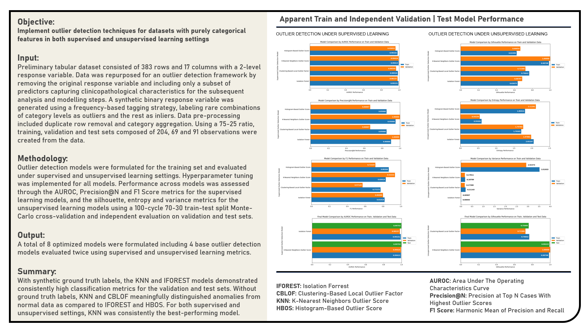
3. References 
- [Book] Applied Predictive Modeling by Max Kuhn and Kjell Johnson
- [Book] An Introduction to Statistical Learning by Gareth James, Daniela Witten, Trevor Hastie and Rob Tibshirani
- [Book] Outlier Analysis by Charu Aggarwal
- [Book] Beginning Anomaly Detection Using Python-Based Deep Learning: With Keras and PyTorch by Sridhar Alla and Suman Kalyan Adari
- [Python Library API] NumPy by NumPy Team
- [Python Library API] pandas by Pandas Team
- [Python Library API] seaborn by Seaborn Team
- [Python Library API] matplotlib.pyplot by MatPlotLib Team
- [Python Library API] matplotlib.image by MatPlotLib Team
- [Python Library API] matplotlib.offsetbox by MatPlotLib Team
- [Python Library API] itertools by Python Team
- [Python Library API] operator by Python Team
- [Python Library API] sklearn.preprocessing by Scikit-Learn Team
- [Python Library API] sklearn.cluster by Scikit-Learn Team
- [Python Library API] sklearn.decomposition by Scikit-Learn Team
- [Python Library API] sklearn.manifold by Scikit-Learn Team
- [Python Library API] sklearn.metrics by Scikit-Learn Team
- [Python Library API] sklearn.model_selection by Scikit-Learn Team
- [Python Library API] StatsModels by StatsModels Team
- [Python Library API] SciPy by SciPy Team
- [Python Library API] pyod by PyOD Team
- [Python Library API] Plotly by Plotly Team
- [Python Library API] umap by Umap-Learn Team
- [Article] Awesome Outlier Detection Resources by Durgesh Samariya (GitHub.Com)
- [Article] Isolation Forest Anomaly Detection — Identify Outliers by Young Yoon (Medium)
- [Article] Isolation Forest Guide: Explanation and Python Implementation by DataCamp Team (DataCamp.Com)
- [Article] Outlier Detection with Isolation Forest by Eryk Lewinson (Towards Data Science)
- [Article] Outlier Detection with Extended Isolation Forest by Eryk Lewinson (Towards Data Science)
- [Article] Isolation Forest for Anomaly Detection by MatLab Team (MathWorks.Com)
- [Article] Unsupervised Outlier Detection with Isolation Forest by Yenwee Lim (Medium)
- [Article] Anomaly Detection with Isolation Forest and Kernel Density Estimation by Muhammad Asad Iqbal Khan (Machine Learning Mastery)
- [Article] Exploring Outlier Handling Techniques: A Comparative Analysis of Isolation Forest, Log-Transformation, and Random Forest on Paris Bike Count Data by Li-Hsiang Hsu (Medium)
- [Article] Isolation Forest – Auto Anomaly Detection with Python by Andy McDonald (Towards Data Science)
- [Article] Local Outlier Factor (LOF) – Algorithm for Outlier Identification by Vaibhav Jayaswal (Towards Data Science)
- [Article] Anomaly Detection with Local Outlier Factor (LOF) by Ilyurek Kilic (Medium)
- [Article] Understanding Local Outlier Factor (LOF) for Anomaly Detection: A Comprehensive Guide with Python Implementation by Shubham Sangole (Medium)
- [Article] An In-depth Guide to Local Outlier Factor (LOF) for Outlier Detection in Python by Alexandra Amidon (Medium)
- [Article] With Python Outlier Detection — KNN by Chris Kuo (Medium)
- [Article] HBOS: Efficient Outlier Detection with Python by Geeks For Geeks Team (GeeksForGeeks.Org)
- [Article] Handbook of Anomaly Detection: with Python Outlier Detection — HBOS by by Chris Kuo (Medium)
- [Article] Intuitive Visualization of Outlier Detection Methods by Matthew Mayo (KDNuggets.Com)
- [Article] Anomaly Detection – How to Tell Good Performance from Bad by Julia Bohutska (Towards Data Science)
- [Publication] Discovering Cluster-Based Local Outliers by Zengyou He, Xiaofei Xu, and Shengchun Deng (Pattern Recognition Letters)
- [Publication] Isolation Forest by Fei Tony Liu, Kai Ming Ting, and Zhi-Hua Zhou (Data Mining, 2008. ICDM'08. Eighth IEEE International Conference)
- [Publication] Isolation-Based Anomaly Detection by Fei Tony Liu, Kai Ming Ting, and Zhi-Hua Zhou (ACM Transactions on Knowledge Discovery from Data (TKDD))
- [Publication] Fast Outlier Detection in High Dimensional Spaces by Fabrizio Angiulli and Clara Pizzuti (European Conference on Principles of Data Mining and Knowledge Discovery)
- [Publication] Efficient Algorithms for Mining Outliers from Large Data Sets by Sridhar Ramaswamy, Rajeev Rastogi, and Kyuseok Shim (ACM Sigmod Record)
- [Publication] Histogram-Based Outlier Score (HBOS): A Fast Unsupervised Anomaly Detection Algorithm by Markus Goldstein and Andreas Dengel (KI-2012: Poster and Demo Track)
- [Video Tutorial] Complete Anomaly Detection Tutorials Machine Learning And Its Types With Implementation by Krish Naik (YouTube)
- [Course] DataCamp Python Data Analyst Certificate by DataCamp Team (DataCamp)
- [Course] DataCamp Python Associate Data Scientist Certificate by DataCamp Team (DataCamp)
- [Course] DataCamp Python Data Scientist Certificate by DataCamp Team (DataCamp)
- [Course] DataCamp Machine Learning Engineer Certificate by DataCamp Team (DataCamp)
- [Course] DataCamp Machine Learning Scientist Certificate by DataCamp Team (DataCamp)
- [Course] IBM Data Analyst Professional Certificate by IBM Team (Coursera)
- [Course] IBM Data Science Professional Certificate by IBM Team (Coursera)
- [Course] IBM Machine Learning Professional Certificate by IBM Team (Coursera)
from IPython.display import display, HTML
display(HTML("<style>.rendered_html { font-size: 15px; font-family: 'Trebuchet MS'; }</style>"))