Model Deployment : Detecting and Analyzing Machine Learning Model Drift Using Open-Source Monitoring Tools
- 1. Table of Contents
- 2. Summary
- 3. References
1. Table of Contents 
This project investigates open-source frameworks for post-deployment model monitoring and performance estimation, with a particular focus on NannyML in detecting and interpreting shifts in machine learning pipelines using Python. The objective was to systematically analyze how different types of drift and distributional changes manifest after model deployment, and to demonstrate how robust monitoring mitigates risks of performance degradation and biased decision-making. The workflow began with the development and selection of a baseline predictive model, which serves as a reference for stability. The dataset was then deliberately perturbed to simulate a range of realistic post-deployment scenarios: Covariate Drift (shifts in feature distributions), Prior Shift (changes in target label proportions), Concept Drift (evolving relationships between features and outcomes), Missingness Spikes (abrupt increases in absent data), and Seasonal Patterns (periodic variations in distributions). NannyML’s Kolmogorov–Smirnov (KS) Statistic and Confidence-Based Performance Estimation (CBPE) Method were subsequently applied to diagnose these shifts, evaluate their potential impact, and provide interpretable insights into model reliability. By contrasting baseline and perturbed conditions, the experiment demonstrated how continuous monitoring augments traditional offline evaluation, offering a safeguard against hidden risks. The findings highlighted how tools like NannyML can integrate seamlessly into MLOps workflows to enable proactive governance, early warning systems, and sustainable deployment practices. All results were consolidated in a Summary presented at the end of the document.
Post-Deployment Monitoring refers to the continuous oversight of machine learning models once they are integrated into production systems. Unlike offline evaluation, which relies on static validation datasets, monitoring addresses the challenges of evolving real-world data streams where underlying distributions may shift. Effective monitoring ensures that models remain accurate, unbiased, and aligned with business objectives. In MLOps, monitoring encompasses data integrity checks, drift detection, performance estimation, and alerting mechanisms. NannyML operationalizes this concept by focusing on performance estimation without ground truth, and by offering statistical methods to detect when data or predictions deviate from expected baselines. The challenges of post-deployment monitoring include delayed or missing ground truth labels, non-stationary data, hidden feedback loops, and difficulties distinguishing natural fluctuations from problematic drifts. Common solutions involve deploying drift detection algorithms, conducting regular audits of data pipelines, simulating counterfactuals, and retraining models on updated data. Monitoring frameworks must balance sensitivity (detecting real problems quickly) with robustness (avoiding false alarms caused by natural noise). Another key challenge is explainability: stakeholders need interpretable signals that justify interventions such as retraining or rolling back models. Tools like NannyML address these challenges through statistical tests for data drift, performance estimation without labels, missingness tracking, and visual diagnostics, making monitoring actionable for data scientists and business teams alike.
Baseline Control represents the stable reference state of a machine learning system against which all post-deployment data and model behavior are compared. It is typically generated using a clean, representative sample of pre-deployment data or early production data collected under known, reliable conditions. This dataset serves as the foundation for defining expected feature distributions, class priors, and performance benchmarks. In post-deployment monitoring, the Baseline Control is essential for distinguishing normal variability from problematic drift or degradation. Metrics such as feature stability, label proportions, and estimated performance consistency characterize its reliability. NannyML operationalizes Baseline Control by allowing users to designate a reference period, fit estimators such as CBPE (Confidence-Based Performance Estimation) on that data, and compute statistical boundaries or confidence intervals. Deviations in subsequent analysis periods, whether in feature distributions, prediction probabilities, or estimated performance, are then detected relative to this baseline. The Baseline Control thus functions as both an empirical anchor and a diagnostic standard, ensuring that drift alerts and performance anomalies are meaningfully contextualized against the model’s original operating state.
Covariate Drift occurs when the distribution of input features changes over time compared to the data used to train the model. Also known as data drift, it does not necessarily imply that the model’s predictive mapping is invalid, but it often precedes performance degradation. Detecting covariate drift requires comparing feature distributions between baseline (reference) data and incoming production data. NannyML provides multiple statistical tests and visualization tools to flag significant changes. Key signatures of covariate drift include shifts in summary statistics, changes in distributional shape, or increased divergence between reference and production feature distributions. These shifts may lead to poor generalization, as the model has not been exposed to the altered feature ranges. Detection techniques include univariate statistical tests (Kolmogorov–Smirnov, Chi-square), multivariate distance measures (Jensen–Shannon divergence, Population Stability Index), and density estimation methods. Remediation approaches involve domain adaptation, re-weighting training samples, or retraining models on updated data distributions. NannyML implements univariate and multivariate tests, provides drift magnitude quantification, and visualizes feature-level changes, allowing practitioners to pinpoint which features are most responsible for the detected drift.
Prior Shift arises when the distribution of the target variable changes, while the conditional relationship between features and labels remains stable. This is also referred to as label shift. Models trained on the original distribution may underperform because their predictions no longer match the new class priors. Detecting prior shifts is crucial, especially in imbalanced classification tasks where small changes in priors can lead to large performance impacts. Prior shift is typically characterized by systematic increases or decreases in class frequencies without corresponding changes in feature distributions. Its impact includes skewed decision thresholds, inflated false positives or false negatives, and degraded calibration of predicted probabilities. Detection approaches include monitoring predicted class proportions, estimating priors using EM-based algorithms, and re-weighting predictions to align with new distributions. Correction strategies may involve resampling, threshold adjustment, or cost-sensitive learning. NannyML assists by tracking predicted probability distributions and comparing them against reference priors, using techniques such as Jensen–Shannon divergence and Population Stability Index to quantify the magnitude of shift.
Concept Drift occurs when the underlying relationship between input features and target labels evolves over time. Unlike covariate drift, where features change independently, concept drift implies that the model’s mapping function itself becomes outdated. Concept drift is among the most damaging forms of drift because it directly undermines predictive accuracy. Detecting it often requires monitoring model outputs or inferred performance over time. NannyML addresses this by estimating performance even when ground truth labels are unavailable. Concept drift is typically signaled by a gradual or sudden decline in performance metrics, inconsistent error patterns, or misalignment between expected and actual prediction behavior. Its impact is severe: models may lose predictive power entirely if they cannot adapt. Detection methods include window-based performance monitoring, hypothesis testing, adaptive ensembles, and statistical monitoring of residuals. Corrective actions include periodic retraining, incremental learning, and online adaptation strategies. NannyML leverages Confidence-Based Performance Estimation (CBPE) and other statistical techniques to estimate performance degradation without labels, making it possible to detect concept drift in real-time production environments.
Missingness Spike refers to sudden increases in missing values within production data. Missing features can destabilize preprocessing pipelines, distort predictions, and signal upstream data collection failures. Monitoring missingness is critical for ensuring both model reliability and data pipeline health. NannyML provides built-in mechanisms to track and visualize changes in missing data patterns, alerting stakeholders before downstream impacts occur. Key indicators of missingness spikes include abrupt rises in null counts, missing categorical levels, or structural breaks in feature completeness. The consequences range from biased predictions to outright system failures if preprocessing pipelines cannot handle unexpected missingness. Detection methods include statistical monitoring of missing value proportions, anomaly detection on completeness metrics, and threshold-based alerts. Solutions typically involve robust imputation, pipeline hardening, and upstream data validation. NannyML offers automated missingness detection, completeness trend visualization, and configurable thresholds, ensuring that missingness issues are surfaced early.
Seasonal Pattern Shift represents periodic fluctuations in data distributions or outcomes that follow predictable cycles. If models are not trained with sufficient historical data to capture these patterns, their predictions may systematically underperform during certain periods. NannyML’s monitoring can reveal recurring deviations, helping teams distinguish between natural seasonality and genuine drift that requires retraining. Seasonality is often characterized by cyclic patterns in data features, prediction distributions, or performance metrics. Its impact includes systematic biases, recurring error peaks, and difficulty distinguishing drift from natural variability. Detection techniques include autocorrelation analysis, Fourier decomposition, and seasonal-trend decomposition. Mitigation strategies involve training with longer historical datasets, adding time-related features, or developing seasonally adaptive models. NannyML highlights recurring deviations in drift metrics, making it easier for practitioners to separate cyclical behavior from true degradation, ensuring that alerts are contextually relevant.
Performance Estimation Without Labels refers to scenarios in real-world deployments where the ground truth often arrives with delays or or may never be available. This makes direct performance tracking difficult. NannyML addresses this challenge by providing algorithms to estimate model performance without labels using confidence distributions, statistical inference, and robust estimation techniques. This capability allows practitioners to maintain visibility into model health continuously, even in label-scarce settings, bridging a critical gap in MLOps monitoring practices. Algorithms in this domain include Confidence-Based Performance Estimation (CBPE), which infers performance by comparing predicted probability distributions against expected confidence intervals, and Direct Loss Estimation, which approximates error rates based on calibration. Statistical inference techniques allow practitioners to construct confidence bounds around estimated metrics, while robust estimation mitigates the risk of spurious signals caused by small sample sizes or noisy predictions. NannyML provides implementations of CBPE and DLE, supporting metrics such as precision, recall, F1-score, and AUROC, all estimated without labels. This makes it possible to detect when a model is underperforming even before labels are collected, reducing blind spots in production monitoring.
Performance Estimation With Labels refers to the direct evaluation of model predictions against actual ground truth outcomes once labels are available. Unlike label-free methods, this approach allows for precise calculation of traditional performance metrics such as accuracy, precision, recall, F1-score, AUROC, and calibration error. Monitoring with labels provides the most reliable indication of model performance, enabling fine-grained diagnosis of errors and biases. The advantage of having labels is the ability to attribute errors to specific subgroups, detect fairness violations, and conduct targeted retraining. Challenges include label delay, annotation quality, and ensuring that labels accurately reflect the operational environment. Common approaches include sliding window evaluation, where performance is tracked over recent data batches, and benchmark comparison, where production metrics are compared to baseline test set results. NannyML incorporates labeled performance tracking alongside its label-free estimators, allowing users to validate estimates once ground truth becomes available. This dual capability ensures consistency, improves confidence in label-free methods, and provides a comprehensive framework for performance monitoring in both short-term and long-term horizons.
1.1. Data Background 
An open Breast Cancer Dataset from Kaggle (with all credits attributed to Wasiq Ali) was used for the analysis as consolidated from the following primary sources:
- Reference Repository entitled Differentiated breast Cancer Recurrence from UC Irvine Machine Learning Repository
- Research Paper entitled Nuclear Feature Extraction for Breast Tumor Diagnosis from the Electronic Imaging
This study hypothesized that the cell nuclei features derived from digitized images of fine needle aspirates (FNA) of breast masses influence breast cancer diagnoses between patients.
The dichotomous categorical variable for the study is:
- diagnosis - Status of the patient (M, Medical diagnosis of a cancerous breast tumor | B, Medical diagnosis of a non-cancerous breast tumor)
The predictor variables for the study are:
- radius_mean - Mean of the radius measurements (Mean of distances from center to points on the perimeter)
- texture_mean - Mean of the texture measurements (Standard deviation of grayscale values)
- perimeter_mean - Mean of the perimeter measurements
- area_mean - Mean of the area measurements
- smoothness_mean - Mean of the smoothness measurements (Local variation in radius lengths)
- compactness_mean - Mean of the compactness measurements (Perimeter² / area - 1.0)
- concavity_mean - Mean of the concavity measurements (Severity of concave portions of the contour)
- concave points_mean - Mean of the concave points measurements (Number of concave portions of the contour)
- symmetry_mean - Mean of the symmetry measurements
- fractal_dimension_mean - Mean of the fractal dimension measurements (Coastline approximation - 1)
- radius_se - Standard error of the radius measurements (Standard error of distances from center to points on the perimeter)
- texture_se - Standard error of the texture measurements (Standard deviation of grayscale values)
- perimeter_se - Standard error of the perimeter measurements
- area_se - Standard error of the area measurements
- smoothness_se - Standard error of the smoothness measurements (Local variation in radius lengths)
- compactness_se - Standard error of the compactness measurements (Perimeter² / area - 1.0)
- concavity_se - Standard error of the concavity measurements (Severity of concave portions of the contour)
- concave points_se - Standard error of the concave points measurements (Number of concave portions of the contour)
- symmetry_se - Standard error of the symmetry measurements
- fractal_dimension_se - Standard error of the fractal dimension measurements (Coastline approximation - 1)
- radius_worst - Largest value of the radius measurements (Largest value of distances from center to points on the perimeter)
- texture_worst - Largest value of the texture measurements (Standard deviation of grayscale values)
- perimeter_worst - Largest value of the perimeter measurements
- area_worst - Largest value of the area measurements
- smoothness_worst - Largest value of the smoothness measurements (Local variation in radius lengths)
- compactness_worst - Largest value of the compactness measurements (Perimeter² / area - 1.0)
- concavity_worst - Largest value of the concavity measurements (Severity of concave portions of the contour)
- concave points_worst - Largest value of the concave points measurements (Number of concave portions of the contour)
- symmetry_worst - Largest value of the symmetry measurements
- fractal_dimension_worst - Largest value of the fractal dimension measurements (Coastline approximation - 1)
1.2. Data Description 
- The initial tabular dataset was comprised of 569 observations and 32 variables (including 1 metadata, 1 target and 30 predictors).
- 569 rows (observations)
- 32 columns (variables)
- 1/32 metadata (categorical)
- id
- 1/32 target (categorical)
- diagnosis
- 30/32 predictor (numeric)
- radius_mean
- texture_mean
- perimeter_mean
- area_mean
- smoothness_mean
- compactness_mean
- concavity_mean
- concave points_mean
- symmetry_mean
- fractal_dimension_mean
- radius_se
- texture_se
- perimeter_se
- area_se
- smoothness_se
- compactness_se
- concavity_se
- concave points_se
- symmetry_se
- fractal_dimension_se
- radius_worst
- texture_worst
- perimeter_worst
- area_worst
- smoothness_worst
- compactness_worst
- concavity_worst
- concave points_worst
- symmetry_worst
- fractal_dimension_worst
- 1/32 metadata (categorical)
- The id variable was transformed to a row index for the data observations.
##################################
# Loading Python Libraries
##################################
import numpy as np
import pandas as pd
import seaborn as sns
import matplotlib.pyplot as plt
import os
import joblib
import re
import pickle
%matplotlib inline
import nannyml as nml
from nannyml.performance_estimation import CBPE
from nannyml.performance_calculation import PerformanceCalculator
from nannyml.chunk import DefaultChunker
import hashlib
import json
from urllib.parse import urlparse
import logging
from operator import truediv
from sklearn.preprocessing import StandardScaler, FunctionTransformer
from sklearn.decomposition import PCA
from scipy import stats
from scipy.stats import pointbiserialr, chi2_contingency
from sklearn.pipeline import Pipeline
from sklearn.compose import ColumnTransformer
from sklearn.tree import DecisionTreeClassifier
from sklearn.ensemble import RandomForestClassifier, AdaBoostClassifier, GradientBoostingClassifier
from sklearn.impute import SimpleImputer
from xgboost import XGBClassifier
from lightgbm import LGBMClassifier
from catboost import CatBoostClassifier
from sklearn.metrics import accuracy_score, precision_score, recall_score, f1_score, roc_auc_score, confusion_matrix, classification_report
from sklearn.model_selection import train_test_split, ParameterGrid, StratifiedShuffleSplit, RepeatedStratifiedKFold, GridSearchCV
from sklearn.utils import resample
from sklearn.base import clone
import warnings
warnings.filterwarnings("ignore", message=".*force_all_finite.*")
warnings.filterwarnings("ignore", message="X does not have valid feature names")
##################################
# Defining file paths
##################################
DATASETS_ORIGINAL_PATH = r"datasets\original"
DATASETS_FINAL_PATH = r"datasets\final\complete"
DATASETS_FINAL_TRAIN_PATH = r"datasets\final\train"
DATASETS_FINAL_TRAIN_FEATURES_PATH = r"datasets\final\train\features"
DATASETS_FINAL_TRAIN_TARGET_PATH = r"datasets\final\train\target"
DATASETS_FINAL_VALIDATION_PATH = r"datasets\final\validation"
DATASETS_FINAL_VALIDATION_FEATURES_PATH = r"datasets\final\validation\features"
DATASETS_FINAL_VALIDATION_TARGET_PATH = r"datasets\final\validation\target"
DATASETS_FINAL_TEST_PATH = r"datasets\final\test"
DATASETS_FINAL_TEST_FEATURES_PATH = r"datasets\final\test\features"
DATASETS_FINAL_TEST_TARGET_PATH = r"datasets\final\test\target"
DATASETS_PREPROCESSED_PATH = r"datasets\preprocessed"
DATASETS_PREPROCESSED_TRAIN_PATH = r"datasets\preprocessed\train"
DATASETS_PREPROCESSED_TRAIN_FEATURES_PATH = r"datasets\preprocessed\train\features"
DATASETS_PREPROCESSED_TRAIN_TARGET_PATH = r"datasets\preprocessed\train\target"
DATASETS_PREPROCESSED_VALIDATION_PATH = r"datasets\preprocessed\validation"
DATASETS_PREPROCESSED_VALIDATION_FEATURES_PATH = r"datasets\preprocessed\validation\features"
DATASETS_PREPROCESSED_VALIDATION_TARGET_PATH = r"datasets\preprocessed\validation\target"
DATASETS_PREPROCESSED_TEST_PATH = r"datasets\preprocessed\test"
DATASETS_PREPROCESSED_TEST_FEATURES_PATH = r"datasets\preprocessed\test\features"
DATASETS_PREPROCESSED_TEST_TARGET_PATH = r"datasets\preprocessed\test\target"
MODELS_PATH = r"models"
##################################
# Loading the dataset
# from the DATASETS_ORIGINAL_PATH
##################################
breast_cancer = pd.read_csv(os.path.join("..", DATASETS_ORIGINAL_PATH, "Breast_Cancer_Dataset.csv"))
##################################
# Performing a general exploration of the dataset
##################################
print('Dataset Dimensions: ')
display(breast_cancer.shape)
Dataset Dimensions:
(569, 32)
##################################
# Listing the column names and data types
##################################
print('Column Names and Data Types:')
display(breast_cancer.dtypes)
Column Names and Data Types:
id int64 diagnosis object radius_mean float64 texture_mean float64 perimeter_mean float64 area_mean float64 smoothness_mean float64 compactness_mean float64 concavity_mean float64 concave points_mean float64 symmetry_mean float64 fractal_dimension_mean float64 radius_se float64 texture_se float64 perimeter_se float64 area_se float64 smoothness_se float64 compactness_se float64 concavity_se float64 concave points_se float64 symmetry_se float64 fractal_dimension_se float64 radius_worst float64 texture_worst float64 perimeter_worst float64 area_worst float64 smoothness_worst float64 compactness_worst float64 concavity_worst float64 concave points_worst float64 symmetry_worst float64 fractal_dimension_worst float64 dtype: object
##################################
# Setting the ID column as row names
##################################
breast_cancer = breast_cancer.set_index("id")
##################################
# Taking a snapshot of the dataset
##################################
breast_cancer.head()
| diagnosis | radius_mean | texture_mean | perimeter_mean | area_mean | smoothness_mean | compactness_mean | concavity_mean | concave points_mean | symmetry_mean | ... | radius_worst | texture_worst | perimeter_worst | area_worst | smoothness_worst | compactness_worst | concavity_worst | concave points_worst | symmetry_worst | fractal_dimension_worst | |
|---|---|---|---|---|---|---|---|---|---|---|---|---|---|---|---|---|---|---|---|---|---|
| id | |||||||||||||||||||||
| 842302 | M | 17.99 | 10.38 | 122.80 | 1001.0 | 0.11840 | 0.27760 | 0.3001 | 0.14710 | 0.2419 | ... | 25.38 | 17.33 | 184.60 | 2019.0 | 0.1622 | 0.6656 | 0.7119 | 0.2654 | 0.4601 | 0.11890 |
| 842517 | M | 20.57 | 17.77 | 132.90 | 1326.0 | 0.08474 | 0.07864 | 0.0869 | 0.07017 | 0.1812 | ... | 24.99 | 23.41 | 158.80 | 1956.0 | 0.1238 | 0.1866 | 0.2416 | 0.1860 | 0.2750 | 0.08902 |
| 84300903 | M | 19.69 | 21.25 | 130.00 | 1203.0 | 0.10960 | 0.15990 | 0.1974 | 0.12790 | 0.2069 | ... | 23.57 | 25.53 | 152.50 | 1709.0 | 0.1444 | 0.4245 | 0.4504 | 0.2430 | 0.3613 | 0.08758 |
| 84348301 | M | 11.42 | 20.38 | 77.58 | 386.1 | 0.14250 | 0.28390 | 0.2414 | 0.10520 | 0.2597 | ... | 14.91 | 26.50 | 98.87 | 567.7 | 0.2098 | 0.8663 | 0.6869 | 0.2575 | 0.6638 | 0.17300 |
| 84358402 | M | 20.29 | 14.34 | 135.10 | 1297.0 | 0.10030 | 0.13280 | 0.1980 | 0.10430 | 0.1809 | ... | 22.54 | 16.67 | 152.20 | 1575.0 | 0.1374 | 0.2050 | 0.4000 | 0.1625 | 0.2364 | 0.07678 |
5 rows × 31 columns
##################################
# Performing a general exploration of the numeric variables
##################################
print('Numeric Variable Summary:')
display(breast_cancer.describe(include='number').transpose())
Numeric Variable Summary:
| count | mean | std | min | 25% | 50% | 75% | max | |
|---|---|---|---|---|---|---|---|---|
| radius_mean | 569.0 | 14.127292 | 3.524049 | 6.981000 | 11.700000 | 13.370000 | 15.780000 | 28.11000 |
| texture_mean | 569.0 | 19.289649 | 4.301036 | 9.710000 | 16.170000 | 18.840000 | 21.800000 | 39.28000 |
| perimeter_mean | 569.0 | 91.969033 | 24.298981 | 43.790000 | 75.170000 | 86.240000 | 104.100000 | 188.50000 |
| area_mean | 569.0 | 654.889104 | 351.914129 | 143.500000 | 420.300000 | 551.100000 | 782.700000 | 2501.00000 |
| smoothness_mean | 569.0 | 0.096360 | 0.014064 | 0.052630 | 0.086370 | 0.095870 | 0.105300 | 0.16340 |
| compactness_mean | 569.0 | 0.104341 | 0.052813 | 0.019380 | 0.064920 | 0.092630 | 0.130400 | 0.34540 |
| concavity_mean | 569.0 | 0.088799 | 0.079720 | 0.000000 | 0.029560 | 0.061540 | 0.130700 | 0.42680 |
| concave points_mean | 569.0 | 0.048919 | 0.038803 | 0.000000 | 0.020310 | 0.033500 | 0.074000 | 0.20120 |
| symmetry_mean | 569.0 | 0.181162 | 0.027414 | 0.106000 | 0.161900 | 0.179200 | 0.195700 | 0.30400 |
| fractal_dimension_mean | 569.0 | 0.062798 | 0.007060 | 0.049960 | 0.057700 | 0.061540 | 0.066120 | 0.09744 |
| radius_se | 569.0 | 0.405172 | 0.277313 | 0.111500 | 0.232400 | 0.324200 | 0.478900 | 2.87300 |
| texture_se | 569.0 | 1.216853 | 0.551648 | 0.360200 | 0.833900 | 1.108000 | 1.474000 | 4.88500 |
| perimeter_se | 569.0 | 2.866059 | 2.021855 | 0.757000 | 1.606000 | 2.287000 | 3.357000 | 21.98000 |
| area_se | 569.0 | 40.337079 | 45.491006 | 6.802000 | 17.850000 | 24.530000 | 45.190000 | 542.20000 |
| smoothness_se | 569.0 | 0.007041 | 0.003003 | 0.001713 | 0.005169 | 0.006380 | 0.008146 | 0.03113 |
| compactness_se | 569.0 | 0.025478 | 0.017908 | 0.002252 | 0.013080 | 0.020450 | 0.032450 | 0.13540 |
| concavity_se | 569.0 | 0.031894 | 0.030186 | 0.000000 | 0.015090 | 0.025890 | 0.042050 | 0.39600 |
| concave points_se | 569.0 | 0.011796 | 0.006170 | 0.000000 | 0.007638 | 0.010930 | 0.014710 | 0.05279 |
| symmetry_se | 569.0 | 0.020542 | 0.008266 | 0.007882 | 0.015160 | 0.018730 | 0.023480 | 0.07895 |
| fractal_dimension_se | 569.0 | 0.003795 | 0.002646 | 0.000895 | 0.002248 | 0.003187 | 0.004558 | 0.02984 |
| radius_worst | 569.0 | 16.269190 | 4.833242 | 7.930000 | 13.010000 | 14.970000 | 18.790000 | 36.04000 |
| texture_worst | 569.0 | 25.677223 | 6.146258 | 12.020000 | 21.080000 | 25.410000 | 29.720000 | 49.54000 |
| perimeter_worst | 569.0 | 107.261213 | 33.602542 | 50.410000 | 84.110000 | 97.660000 | 125.400000 | 251.20000 |
| area_worst | 569.0 | 880.583128 | 569.356993 | 185.200000 | 515.300000 | 686.500000 | 1084.000000 | 4254.00000 |
| smoothness_worst | 569.0 | 0.132369 | 0.022832 | 0.071170 | 0.116600 | 0.131300 | 0.146000 | 0.22260 |
| compactness_worst | 569.0 | 0.254265 | 0.157336 | 0.027290 | 0.147200 | 0.211900 | 0.339100 | 1.05800 |
| concavity_worst | 569.0 | 0.272188 | 0.208624 | 0.000000 | 0.114500 | 0.226700 | 0.382900 | 1.25200 |
| concave points_worst | 569.0 | 0.114606 | 0.065732 | 0.000000 | 0.064930 | 0.099930 | 0.161400 | 0.29100 |
| symmetry_worst | 569.0 | 0.290076 | 0.061867 | 0.156500 | 0.250400 | 0.282200 | 0.317900 | 0.66380 |
| fractal_dimension_worst | 569.0 | 0.083946 | 0.018061 | 0.055040 | 0.071460 | 0.080040 | 0.092080 | 0.20750 |
1.3. Data Quality Assessment 
Data quality findings based on assessment are as follows:
- No duplicated rows were noted.
- No missing data noted for any variable with Null.Count>0 and Fill.Rate<1.0.
- No low variance observed for any variable with First.Second.Mode.Ratio>5.
- No low variance observed for any variable with Unique.Count.Ratio>10.
- High skewness observed for 5 variables with Skewness>3 or Skewness<(-3).
- area_se: Skewness = 5.447
- concavity_se: Skewness = 5.110
- fractal_dimension_se: Skewness = 3.923
- perimeter_se: Skewness = 3.443
- radius_se: Skewness = 3.088
##################################
# Counting the number of duplicated rows
##################################
breast_cancer.duplicated().sum()
np.int64(0)
##################################
# Gathering the data types for each column
##################################
data_type_list = list(breast_cancer.dtypes)
##################################
# Gathering the variable names for each column
##################################
variable_name_list = list(breast_cancer.columns)
##################################
# Gathering the number of observations for each column
##################################
row_count_list = list([len(breast_cancer)] * len(breast_cancer.columns))
##################################
# Gathering the number of missing data for each column
##################################
null_count_list = list(breast_cancer.isna().sum(axis=0))
##################################
# Gathering the number of non-missing data for each column
##################################
non_null_count_list = list(breast_cancer.count())
##################################
# Gathering the missing data percentage for each column
##################################
fill_rate_list = map(truediv, non_null_count_list, row_count_list)
##################################
# Formulating the summary
# for all columns
##################################
all_column_quality_summary = pd.DataFrame(zip(variable_name_list,
data_type_list,
row_count_list,
non_null_count_list,
null_count_list,
fill_rate_list),
columns=['Column.Name',
'Column.Type',
'Row.Count',
'Non.Null.Count',
'Null.Count',
'Fill.Rate'])
display(all_column_quality_summary)
| Column.Name | Column.Type | Row.Count | Non.Null.Count | Null.Count | Fill.Rate | |
|---|---|---|---|---|---|---|
| 0 | diagnosis | object | 569 | 569 | 0 | 1.0 |
| 1 | radius_mean | float64 | 569 | 569 | 0 | 1.0 |
| 2 | texture_mean | float64 | 569 | 569 | 0 | 1.0 |
| 3 | perimeter_mean | float64 | 569 | 569 | 0 | 1.0 |
| 4 | area_mean | float64 | 569 | 569 | 0 | 1.0 |
| 5 | smoothness_mean | float64 | 569 | 569 | 0 | 1.0 |
| 6 | compactness_mean | float64 | 569 | 569 | 0 | 1.0 |
| 7 | concavity_mean | float64 | 569 | 569 | 0 | 1.0 |
| 8 | concave points_mean | float64 | 569 | 569 | 0 | 1.0 |
| 9 | symmetry_mean | float64 | 569 | 569 | 0 | 1.0 |
| 10 | fractal_dimension_mean | float64 | 569 | 569 | 0 | 1.0 |
| 11 | radius_se | float64 | 569 | 569 | 0 | 1.0 |
| 12 | texture_se | float64 | 569 | 569 | 0 | 1.0 |
| 13 | perimeter_se | float64 | 569 | 569 | 0 | 1.0 |
| 14 | area_se | float64 | 569 | 569 | 0 | 1.0 |
| 15 | smoothness_se | float64 | 569 | 569 | 0 | 1.0 |
| 16 | compactness_se | float64 | 569 | 569 | 0 | 1.0 |
| 17 | concavity_se | float64 | 569 | 569 | 0 | 1.0 |
| 18 | concave points_se | float64 | 569 | 569 | 0 | 1.0 |
| 19 | symmetry_se | float64 | 569 | 569 | 0 | 1.0 |
| 20 | fractal_dimension_se | float64 | 569 | 569 | 0 | 1.0 |
| 21 | radius_worst | float64 | 569 | 569 | 0 | 1.0 |
| 22 | texture_worst | float64 | 569 | 569 | 0 | 1.0 |
| 23 | perimeter_worst | float64 | 569 | 569 | 0 | 1.0 |
| 24 | area_worst | float64 | 569 | 569 | 0 | 1.0 |
| 25 | smoothness_worst | float64 | 569 | 569 | 0 | 1.0 |
| 26 | compactness_worst | float64 | 569 | 569 | 0 | 1.0 |
| 27 | concavity_worst | float64 | 569 | 569 | 0 | 1.0 |
| 28 | concave points_worst | float64 | 569 | 569 | 0 | 1.0 |
| 29 | symmetry_worst | float64 | 569 | 569 | 0 | 1.0 |
| 30 | fractal_dimension_worst | float64 | 569 | 569 | 0 | 1.0 |
##################################
# Counting the number of columns
# with Fill.Rate < 1.00
##################################
len(all_column_quality_summary[(all_column_quality_summary['Fill.Rate']<1)])
0
##################################
# Identifying the rows
# with Fill.Rate < 0.90
##################################
column_low_fill_rate = all_column_quality_summary[(all_column_quality_summary['Fill.Rate']<0.90)]
##################################
# Gathering the indices for each observation
##################################
row_index_list = breast_cancer.index
##################################
# Gathering the number of columns for each observation
##################################
column_count_list = list([len(breast_cancer.columns)] * len(breast_cancer))
##################################
# Gathering the number of missing data for each row
##################################
null_row_list = list(breast_cancer.isna().sum(axis=1))
##################################
# Gathering the missing data percentage for each column
##################################
missing_rate_list = map(truediv, null_row_list, column_count_list)
##################################
# Identifying the rows
# with missing data
##################################
all_row_quality_summary = pd.DataFrame(zip(row_index_list,
column_count_list,
null_row_list,
missing_rate_list),
columns=['Row.Name',
'Column.Count',
'Null.Count',
'Missing.Rate'])
display(all_row_quality_summary)
| Row.Name | Column.Count | Null.Count | Missing.Rate | |
|---|---|---|---|---|
| 0 | 842302 | 31 | 0 | 0.0 |
| 1 | 842517 | 31 | 0 | 0.0 |
| 2 | 84300903 | 31 | 0 | 0.0 |
| 3 | 84348301 | 31 | 0 | 0.0 |
| 4 | 84358402 | 31 | 0 | 0.0 |
| ... | ... | ... | ... | ... |
| 564 | 926424 | 31 | 0 | 0.0 |
| 565 | 926682 | 31 | 0 | 0.0 |
| 566 | 926954 | 31 | 0 | 0.0 |
| 567 | 927241 | 31 | 0 | 0.0 |
| 568 | 92751 | 31 | 0 | 0.0 |
569 rows × 4 columns
##################################
# Counting the number of rows
# with Missing.Rate > 0.00
##################################
len(all_row_quality_summary[(all_row_quality_summary['Missing.Rate']>0.00)])
0
##################################
# Formulating the dataset
# with numeric columns only
##################################
breast_cancer_numeric = breast_cancer.select_dtypes(include='number')
##################################
# Gathering the variable names for each numeric column
##################################
numeric_variable_name_list = breast_cancer_numeric.columns
##################################
# Gathering the minimum value for each numeric column
##################################
numeric_minimum_list = breast_cancer_numeric.min()
##################################
# Gathering the mean value for each numeric column
##################################
numeric_mean_list = breast_cancer_numeric.mean()
##################################
# Gathering the median value for each numeric column
##################################
numeric_median_list = breast_cancer_numeric.median()
##################################
# Gathering the maximum value for each numeric column
##################################
numeric_maximum_list = breast_cancer_numeric.max()
##################################
# Gathering the first mode values for each numeric column
##################################
numeric_first_mode_list = [breast_cancer[x].value_counts(dropna=True).index.tolist()[0] for x in breast_cancer_numeric]
##################################
# Gathering the second mode values for each numeric column
##################################
numeric_second_mode_list = [breast_cancer[x].value_counts(dropna=True).index.tolist()[1] for x in breast_cancer_numeric]
##################################
# Gathering the count of first mode values for each numeric column
##################################
numeric_first_mode_count_list = [breast_cancer_numeric[x].isin([breast_cancer[x].value_counts(dropna=True).index.tolist()[0]]).sum() for x in breast_cancer_numeric]
##################################
# Gathering the count of second mode values for each numeric column
##################################
numeric_second_mode_count_list = [breast_cancer_numeric[x].isin([breast_cancer[x].value_counts(dropna=True).index.tolist()[1]]).sum() for x in breast_cancer_numeric]
##################################
# Gathering the first mode to second mode ratio for each numeric column
##################################
numeric_first_second_mode_ratio_list = map(truediv, numeric_first_mode_count_list, numeric_second_mode_count_list)
##################################
# Gathering the count of unique values for each numeric column
##################################
numeric_unique_count_list = breast_cancer_numeric.nunique(dropna=True)
##################################
# Gathering the number of observations for each numeric column
##################################
numeric_row_count_list = list([len(breast_cancer_numeric)] * len(breast_cancer_numeric.columns))
##################################
# Gathering the unique to count ratio for each numeric column
##################################
numeric_unique_count_ratio_list = map(truediv, numeric_unique_count_list, numeric_row_count_list)
##################################
# Gathering the skewness value for each numeric column
##################################
numeric_skewness_list = breast_cancer_numeric.skew()
##################################
# Gathering the kurtosis value for each numeric column
##################################
numeric_kurtosis_list = breast_cancer_numeric.kurtosis()
##################################
# Generating a column quality summary for the numeric column
##################################
numeric_column_quality_summary = pd.DataFrame(zip(numeric_variable_name_list,
numeric_minimum_list,
numeric_mean_list,
numeric_median_list,
numeric_maximum_list,
numeric_first_mode_list,
numeric_second_mode_list,
numeric_first_mode_count_list,
numeric_second_mode_count_list,
numeric_first_second_mode_ratio_list,
numeric_unique_count_list,
numeric_row_count_list,
numeric_unique_count_ratio_list,
numeric_skewness_list,
numeric_kurtosis_list),
columns=['Numeric.Column.Name',
'Minimum',
'Mean',
'Median',
'Maximum',
'First.Mode',
'Second.Mode',
'First.Mode.Count',
'Second.Mode.Count',
'First.Second.Mode.Ratio',
'Unique.Count',
'Row.Count',
'Unique.Count.Ratio',
'Skewness',
'Kurtosis'])
display(numeric_column_quality_summary)
| Numeric.Column.Name | Minimum | Mean | Median | Maximum | First.Mode | Second.Mode | First.Mode.Count | Second.Mode.Count | First.Second.Mode.Ratio | Unique.Count | Row.Count | Unique.Count.Ratio | Skewness | Kurtosis | |
|---|---|---|---|---|---|---|---|---|---|---|---|---|---|---|---|
| 0 | radius_mean | 6.981000 | 14.127292 | 13.370000 | 28.11000 | 12.340000 | 11.060000 | 4 | 3 | 1.333333 | 456 | 569 | 0.801406 | 0.942380 | 0.845522 |
| 1 | texture_mean | 9.710000 | 19.289649 | 18.840000 | 39.28000 | 16.840000 | 19.830000 | 3 | 3 | 1.000000 | 479 | 569 | 0.841828 | 0.650450 | 0.758319 |
| 2 | perimeter_mean | 43.790000 | 91.969033 | 86.240000 | 188.50000 | 82.610000 | 134.700000 | 3 | 3 | 1.000000 | 522 | 569 | 0.917399 | 0.990650 | 0.972214 |
| 3 | area_mean | 143.500000 | 654.889104 | 551.100000 | 2501.00000 | 512.200000 | 394.100000 | 3 | 2 | 1.500000 | 539 | 569 | 0.947276 | 1.645732 | 3.652303 |
| 4 | smoothness_mean | 0.052630 | 0.096360 | 0.095870 | 0.16340 | 0.100700 | 0.105400 | 5 | 4 | 1.250000 | 474 | 569 | 0.833040 | 0.456324 | 0.855975 |
| 5 | compactness_mean | 0.019380 | 0.104341 | 0.092630 | 0.34540 | 0.114700 | 0.120600 | 3 | 3 | 1.000000 | 537 | 569 | 0.943761 | 1.190123 | 1.650130 |
| 6 | concavity_mean | 0.000000 | 0.088799 | 0.061540 | 0.42680 | 0.000000 | 0.120400 | 13 | 3 | 4.333333 | 537 | 569 | 0.943761 | 1.401180 | 1.998638 |
| 7 | concave points_mean | 0.000000 | 0.048919 | 0.033500 | 0.20120 | 0.000000 | 0.028640 | 13 | 3 | 4.333333 | 542 | 569 | 0.952548 | 1.171180 | 1.066556 |
| 8 | symmetry_mean | 0.106000 | 0.181162 | 0.179200 | 0.30400 | 0.176900 | 0.189300 | 4 | 4 | 1.000000 | 432 | 569 | 0.759227 | 0.725609 | 1.287933 |
| 9 | fractal_dimension_mean | 0.049960 | 0.062798 | 0.061540 | 0.09744 | 0.067820 | 0.061130 | 3 | 3 | 1.000000 | 499 | 569 | 0.876977 | 1.304489 | 3.005892 |
| 10 | radius_se | 0.111500 | 0.405172 | 0.324200 | 2.87300 | 0.286000 | 0.220400 | 3 | 3 | 1.000000 | 540 | 569 | 0.949033 | 3.088612 | 17.686726 |
| 11 | texture_se | 0.360200 | 1.216853 | 1.108000 | 4.88500 | 0.856100 | 1.350000 | 3 | 3 | 1.000000 | 519 | 569 | 0.912127 | 1.646444 | 5.349169 |
| 12 | perimeter_se | 0.757000 | 2.866059 | 2.287000 | 21.98000 | 1.778000 | 1.143000 | 4 | 2 | 2.000000 | 533 | 569 | 0.936731 | 3.443615 | 21.401905 |
| 13 | area_se | 6.802000 | 40.337079 | 24.530000 | 542.20000 | 16.970000 | 16.640000 | 3 | 3 | 1.000000 | 528 | 569 | 0.927944 | 5.447186 | 49.209077 |
| 14 | smoothness_se | 0.001713 | 0.007041 | 0.006380 | 0.03113 | 0.005910 | 0.006064 | 2 | 2 | 1.000000 | 547 | 569 | 0.961336 | 2.314450 | 10.469840 |
| 15 | compactness_se | 0.002252 | 0.025478 | 0.020450 | 0.13540 | 0.018120 | 0.011040 | 3 | 3 | 1.000000 | 541 | 569 | 0.950791 | 1.902221 | 5.106252 |
| 16 | concavity_se | 0.000000 | 0.031894 | 0.025890 | 0.39600 | 0.000000 | 0.021850 | 13 | 2 | 6.500000 | 533 | 569 | 0.936731 | 5.110463 | 48.861395 |
| 17 | concave points_se | 0.000000 | 0.011796 | 0.010930 | 0.05279 | 0.000000 | 0.011670 | 13 | 3 | 4.333333 | 507 | 569 | 0.891037 | 1.444678 | 5.126302 |
| 18 | symmetry_se | 0.007882 | 0.020542 | 0.018730 | 0.07895 | 0.013440 | 0.020450 | 4 | 3 | 1.333333 | 498 | 569 | 0.875220 | 2.195133 | 7.896130 |
| 19 | fractal_dimension_se | 0.000895 | 0.003795 | 0.003187 | 0.02984 | 0.002256 | 0.002205 | 2 | 2 | 1.000000 | 545 | 569 | 0.957821 | 3.923969 | 26.280847 |
| 20 | radius_worst | 7.930000 | 16.269190 | 14.970000 | 36.04000 | 12.360000 | 13.500000 | 5 | 4 | 1.250000 | 457 | 569 | 0.803163 | 1.103115 | 0.944090 |
| 21 | texture_worst | 12.020000 | 25.677223 | 25.410000 | 49.54000 | 17.700000 | 27.260000 | 3 | 3 | 1.000000 | 511 | 569 | 0.898067 | 0.498321 | 0.224302 |
| 22 | perimeter_worst | 50.410000 | 107.261213 | 97.660000 | 251.20000 | 117.700000 | 105.900000 | 3 | 3 | 1.000000 | 514 | 569 | 0.903339 | 1.128164 | 1.070150 |
| 23 | area_worst | 185.200000 | 880.583128 | 686.500000 | 4254.00000 | 698.800000 | 808.900000 | 2 | 2 | 1.000000 | 544 | 569 | 0.956063 | 1.859373 | 4.396395 |
| 24 | smoothness_worst | 0.071170 | 0.132369 | 0.131300 | 0.22260 | 0.140100 | 0.131200 | 4 | 4 | 1.000000 | 411 | 569 | 0.722320 | 0.415426 | 0.517825 |
| 25 | compactness_worst | 0.027290 | 0.254265 | 0.211900 | 1.05800 | 0.148600 | 0.341600 | 3 | 3 | 1.000000 | 529 | 569 | 0.929701 | 1.473555 | 3.039288 |
| 26 | concavity_worst | 0.000000 | 0.272188 | 0.226700 | 1.25200 | 0.000000 | 0.450400 | 13 | 3 | 4.333333 | 539 | 569 | 0.947276 | 1.150237 | 1.615253 |
| 27 | concave points_worst | 0.000000 | 0.114606 | 0.099930 | 0.29100 | 0.000000 | 0.110500 | 13 | 3 | 4.333333 | 492 | 569 | 0.864675 | 0.492616 | -0.535535 |
| 28 | symmetry_worst | 0.156500 | 0.290076 | 0.282200 | 0.66380 | 0.236900 | 0.310900 | 3 | 3 | 1.000000 | 500 | 569 | 0.878735 | 1.433928 | 4.444560 |
| 29 | fractal_dimension_worst | 0.055040 | 0.083946 | 0.080040 | 0.20750 | 0.074270 | 0.087010 | 3 | 2 | 1.500000 | 535 | 569 | 0.940246 | 1.662579 | 5.244611 |
##################################
# Counting the number of numeric columns
# with First.Second.Mode.Ratio > 5.00
##################################
len(numeric_column_quality_summary[(numeric_column_quality_summary['First.Second.Mode.Ratio']>10)])
0
##################################
# Counting the number of numeric columns
# with Unique.Count.Ratio > 10.00
##################################
len(numeric_column_quality_summary[(numeric_column_quality_summary['Unique.Count.Ratio']>10)])
0
#################################
# Counting the number of numeric columns
# with Skewness > 3.00 or Skewness < -3.00
##################################
len(numeric_column_quality_summary[(numeric_column_quality_summary['Skewness']>3) | (numeric_column_quality_summary['Skewness']<(-3))])
5
##################################
# Identifying the numerical columns
# with Skewness > 3.00 or Skewness < -3.00
##################################
display(numeric_column_quality_summary[(numeric_column_quality_summary['Skewness']>3) | (numeric_column_quality_summary['Skewness']<(-3))].sort_values(by=['Skewness'], ascending=False))
| Numeric.Column.Name | Minimum | Mean | Median | Maximum | First.Mode | Second.Mode | First.Mode.Count | Second.Mode.Count | First.Second.Mode.Ratio | Unique.Count | Row.Count | Unique.Count.Ratio | Skewness | Kurtosis | |
|---|---|---|---|---|---|---|---|---|---|---|---|---|---|---|---|
| 13 | area_se | 6.802000 | 40.337079 | 24.530000 | 542.20000 | 16.970000 | 16.640000 | 3 | 3 | 1.0 | 528 | 569 | 0.927944 | 5.447186 | 49.209077 |
| 16 | concavity_se | 0.000000 | 0.031894 | 0.025890 | 0.39600 | 0.000000 | 0.021850 | 13 | 2 | 6.5 | 533 | 569 | 0.936731 | 5.110463 | 48.861395 |
| 19 | fractal_dimension_se | 0.000895 | 0.003795 | 0.003187 | 0.02984 | 0.002256 | 0.002205 | 2 | 2 | 1.0 | 545 | 569 | 0.957821 | 3.923969 | 26.280847 |
| 12 | perimeter_se | 0.757000 | 2.866059 | 2.287000 | 21.98000 | 1.778000 | 1.143000 | 4 | 2 | 2.0 | 533 | 569 | 0.936731 | 3.443615 | 21.401905 |
| 10 | radius_se | 0.111500 | 0.405172 | 0.324200 | 2.87300 | 0.286000 | 0.220400 | 3 | 3 | 1.0 | 540 | 569 | 0.949033 | 3.088612 | 17.686726 |
##################################
# Formulating the dataset
# with categorical columns only
##################################
breast_cancer_categorical = breast_cancer.select_dtypes(include=['category','object'])
##################################
# Gathering the variable names for the categorical column
##################################
categorical_variable_name_list = breast_cancer_categorical.columns
##################################
# Gathering the first mode values for each categorical column
##################################
categorical_first_mode_list = [breast_cancer[x].value_counts().index.tolist()[0] for x in breast_cancer_categorical]
##################################
# Gathering the second mode values for each categorical column
##################################
categorical_second_mode_list = [breast_cancer[x].value_counts().index.tolist()[1] for x in breast_cancer_categorical]
##################################
# Gathering the count of first mode values for each categorical column
##################################
categorical_first_mode_count_list = [breast_cancer_categorical[x].isin([breast_cancer[x].value_counts(dropna=True).index.tolist()[0]]).sum() for x in breast_cancer_categorical]
##################################
# Gathering the count of second mode values for each categorical column
##################################
categorical_second_mode_count_list = [breast_cancer_categorical[x].isin([breast_cancer[x].value_counts(dropna=True).index.tolist()[1]]).sum() for x in breast_cancer_categorical]
##################################
# Gathering the first mode to second mode ratio for each categorical column
##################################
categorical_first_second_mode_ratio_list = map(truediv, categorical_first_mode_count_list, categorical_second_mode_count_list)
##################################
# Gathering the count of unique values for each categorical column
##################################
categorical_unique_count_list = breast_cancer_categorical.nunique(dropna=True)
##################################
# Gathering the number of observations for each categorical column
##################################
categorical_row_count_list = list([len(breast_cancer_categorical)] * len(breast_cancer_categorical.columns))
##################################
# Gathering the unique to count ratio for each categorical column
##################################
categorical_unique_count_ratio_list = map(truediv, categorical_unique_count_list, categorical_row_count_list)
##################################
# Generating a column quality summary for the categorical columns
##################################
categorical_column_quality_summary = pd.DataFrame(zip(categorical_variable_name_list,
categorical_first_mode_list,
categorical_second_mode_list,
categorical_first_mode_count_list,
categorical_second_mode_count_list,
categorical_first_second_mode_ratio_list,
categorical_unique_count_list,
categorical_row_count_list,
categorical_unique_count_ratio_list),
columns=['Categorical.Column.Name',
'First.Mode',
'Second.Mode',
'First.Mode.Count',
'Second.Mode.Count',
'First.Second.Mode.Ratio',
'Unique.Count',
'Row.Count',
'Unique.Count.Ratio'])
display(categorical_column_quality_summary)
| Categorical.Column.Name | First.Mode | Second.Mode | First.Mode.Count | Second.Mode.Count | First.Second.Mode.Ratio | Unique.Count | Row.Count | Unique.Count.Ratio | |
|---|---|---|---|---|---|---|---|---|---|
| 0 | diagnosis | B | M | 357 | 212 | 1.683962 | 2 | 569 | 0.003515 |
##################################
# Counting the number of categorical columns
# with First.Second.Mode.Ratio > 5.00
##################################
len(categorical_column_quality_summary[(categorical_column_quality_summary['First.Second.Mode.Ratio']>5)])
0
##################################
# Counting the number of categorical columns
# with Unique.Count.Ratio > 10.00
##################################
len(categorical_column_quality_summary[(categorical_column_quality_summary['Unique.Count.Ratio']>10)])
0
1.4. Data Preprocessing 
1.4.1 Data Splitting
- The baseline dataset is comprised of:
- 569 rows (observations)
- 357 diagnosis=B: 62.74%
- 212 diagnosis=M: 37.26%
- 31 columns (variables)
- 1/31 target (categorical)
- diagnosis
- 30/31 predictor (numeric)
- radius_mean
- texture_mean
- perimeter_mean
- area_mean
- smoothness_mean
- compactness_mean
- concavity_mean
- concave points_mean
- symmetry_mean
- fractal_dimension_mean
- radius_se
- texture_se
- perimeter_se
- area_se
- smoothness_se
- compactness_se
- concavity_se
- concave points_se
- symmetry_se
- fractal_dimension_se
- radius_worst
- texture_worst
- perimeter_worst
- area_worst
- smoothness_worst
- compactness_worst
- concavity_worst
- concave points_worst
- symmetry_worst
- fractal_dimension_worst
- 1/31 target (categorical)
- 569 rows (observations)
- The baseline dataset was divided into three subsets using a fixed random seed:
- test data: 25% of the original data with class stratification applied
- train data (initial): 75% of the original data with class stratification applied
- train data (final): 75% of the train (initial) data with class stratification applied
- validation data: 25% of the train (initial) data with class stratification applied
- Models were developed from the train data (final). Using the same dataset, a subset of models with optimal hyperparameters were selected, based on cross-validation.
- Among candidate models with optimal hyperparameters, the final model was selected based on performance on the validation data.
- Performance of the selected final model (and other candidate models for post-model selection comparison) were evaluated using the test data.
- The train data (final) subset is comprised of:
- 319 rows (observations)
- 200 diagnosis=B: 62.69%
- 119 diagnosis=M: 37.30%
- 31 columns (variables)
- 319 rows (observations)
- The validation data subset is comprised of:
- 107 rows (observations)
- 67 diagnosis=B: 62.61%
- 40 diagnosis=M: 37.38%
- 31 columns (variables)
- 107 rows (observations)
- The test data subset is comprised of:
- 143 rows (observations)
- 90 diagnosis=B: 62.93%
- 53 diagnosis=M: 37.06%
- 31 columns (variables)
- 143 rows (observations)
##################################
# Creating a dataset copy
# of the original data
##################################
breast_cancer_baseline = breast_cancer.copy()
##################################
# Performing a general exploration
# of the baseline dataset
##################################
print('Final Dataset Dimensions: ')
display(breast_cancer_baseline.shape)
Final Dataset Dimensions:
(569, 31)
##################################
# Obtaining the distribution of
# of the target variable
##################################
print('Target Variable Breakdown: ')
breast_cancer_breakdown = breast_cancer_baseline.groupby('diagnosis', observed=True).size().reset_index(name='Count')
breast_cancer_breakdown['Percentage'] = (breast_cancer_breakdown['Count'] / len(breast_cancer_baseline)) * 100
display(breast_cancer_breakdown)
Target Variable Breakdown:
| diagnosis | Count | Percentage | |
|---|---|---|---|
| 0 | B | 357 | 62.741652 |
| 1 | M | 212 | 37.258348 |
##################################
# Formulating the train and test data
# from the final dataset
# by applying stratification and
# using a 75-25 ratio
##################################
breast_cancer_train_initial, breast_cancer_test = train_test_split(breast_cancer_baseline,
test_size=0.25,
stratify=breast_cancer_baseline['diagnosis'],
random_state=987654321)
##################################
# Performing a general exploration
# of the initial training dataset
##################################
X_train_initial = breast_cancer_train_initial.drop('diagnosis', axis = 1)
y_train_initial = breast_cancer_train_initial['diagnosis']
print('Initial Train Dataset Dimensions: ')
display(X_train_initial.shape)
display(y_train_initial.shape)
print('Initial Train Target Variable Breakdown: ')
display(y_train_initial.value_counts())
print('Initial Train Target Variable Proportion: ')
display(y_train_initial.value_counts(normalize = True))
Initial Train Dataset Dimensions:
(426, 30)
(426,)
Initial Train Target Variable Breakdown:
diagnosis B 267 M 159 Name: count, dtype: int64
Initial Train Target Variable Proportion:
diagnosis B 0.626761 M 0.373239 Name: proportion, dtype: float64
##################################
# Performing a general exploration
# of the test dataset
##################################
X_test = breast_cancer_test.drop('diagnosis', axis = 1)
y_test = breast_cancer_test['diagnosis']
print('Test Dataset Dimensions: ')
display(X_test.shape)
display(y_test.shape)
print('Test Target Variable Breakdown: ')
display(y_test.value_counts())
print('Test Target Variable Proportion: ')
display(y_test.value_counts(normalize = True))
Test Dataset Dimensions:
(143, 30)
(143,)
Test Target Variable Breakdown:
diagnosis B 90 M 53 Name: count, dtype: int64
Test Target Variable Proportion:
diagnosis B 0.629371 M 0.370629 Name: proportion, dtype: float64
##################################
# Formulating the train and validation data
# from the train dataset
# by applying stratification and
# using a 75-25 ratio
##################################
breast_cancer_train, breast_cancer_validation = train_test_split(breast_cancer_train_initial,
test_size=0.25,
stratify=breast_cancer_train_initial['diagnosis'],
random_state=987654321)
##################################
# Performing a general exploration
# of the final training dataset
##################################
X_train = breast_cancer_train.drop('diagnosis', axis = 1)
y_train = breast_cancer_train['diagnosis']
print('Final Train Dataset Dimensions: ')
display(X_train.shape)
display(y_train.shape)
print('Final Train Target Variable Breakdown: ')
display(y_train.value_counts())
print('Final Train Target Variable Proportion: ')
display(y_train.value_counts(normalize = True))
Final Train Dataset Dimensions:
(319, 30)
(319,)
Final Train Target Variable Breakdown:
diagnosis B 200 M 119 Name: count, dtype: int64
Final Train Target Variable Proportion:
diagnosis B 0.626959 M 0.373041 Name: proportion, dtype: float64
##################################
# Performing a general exploration
# of the validation dataset
##################################
X_validation = breast_cancer_validation.drop('diagnosis', axis = 1)
y_validation = breast_cancer_validation['diagnosis']
print('Validation Dataset Dimensions: ')
display(X_validation.shape)
display(y_validation.shape)
print('Validation Target Variable Breakdown: ')
display(y_validation.value_counts())
print('Validation Target Variable Proportion: ')
display(y_validation.value_counts(normalize = True))
Validation Dataset Dimensions:
(107, 30)
(107,)
Validation Target Variable Breakdown:
diagnosis B 67 M 40 Name: count, dtype: int64
Validation Target Variable Proportion:
diagnosis B 0.626168 M 0.373832 Name: proportion, dtype: float64
##################################
# Saving the training data
# to the DATASETS_FINAL_TRAIN_PATH
# and DATASETS_FINAL_TRAIN_FEATURES_PATH
# and DATASETS_FINAL_TRAIN_TARGET_PATH
##################################
breast_cancer_train.to_csv(os.path.join("..", DATASETS_FINAL_TRAIN_PATH, "breast_cancer_train.csv"), index=False)
X_train.to_csv(os.path.join("..", DATASETS_FINAL_TRAIN_FEATURES_PATH, "X_train.csv"), index=False)
y_train.to_csv(os.path.join("..", DATASETS_FINAL_TRAIN_TARGET_PATH, "y_train.csv"), index=False)
##################################
# Saving the validation data
# to the DATASETS_FINAL_VALIDATION_PATH
# and DATASETS_FINAL_VALIDATION_FEATURE_PATH
# and DATASETS_FINAL_VALIDATION_TARGET_PATH
##################################
breast_cancer_validation.to_csv(os.path.join("..", DATASETS_FINAL_VALIDATION_PATH, "breast_cancer_validation.csv"), index=False)
X_validation.to_csv(os.path.join("..", DATASETS_FINAL_VALIDATION_FEATURES_PATH, "X_validation.csv"), index=False)
y_validation.to_csv(os.path.join("..", DATASETS_FINAL_VALIDATION_TARGET_PATH, "y_validation.csv"), index=False)
##################################
# Saving the test data
# to the DATASETS_FINAL_TEST_PATH
# and DATASETS_FINAL_TEST_FEATURES_PATH
# and DATASETS_FINAL_TEST_TARGET_PATH
##################################
breast_cancer_test.to_csv(os.path.join("..", DATASETS_FINAL_TEST_PATH, "breast_cancer_test.csv"), index=False)
X_test.to_csv(os.path.join("..", DATASETS_FINAL_TEST_FEATURES_PATH, "X_test.csv"), index=False)
y_test.to_csv(os.path.join("..", DATASETS_FINAL_TEST_TARGET_PATH, "y_test.csv"), index=False)
1.4.2 Outlier and Distributional Shape Analysis
Outlier and distributional shape analysis findings based on assessment of the training data are as follows:
- High skewness observed for 5 variables with Skewness>3 or Skewness<(-3).
- area_se: Skewness = 6.562
- concavity_se: Skewness = 5.648
- fractal_dimension_se: Skewness = 4.280
- perimeter_se: Skewness = 4.136
- radius_se: Skewness = 3.775
- Relatively high number of outliers observed for 7 numeric variables with Outlier.Ratio>0.05.
- area_se: Outlier.Ratio = 0.110
- radius_se: Outlier.Ratio = 0.075
- perimeter_se: Outlier.Ratio = 0.075
- smoothness_se: Outlier.Ratio = 0.059
- compactness_se: Outlier.Ratio = 0.059
- fractal_dimension_se: Outlier.Ratio = 0.056
- symmetry_se: Outlier.Ratio = 0.050
##################################
# Formulating the training dataset
# with numeric columns only
##################################
breast_cancer_train_numeric = breast_cancer_train.select_dtypes(include='number')
##################################
# Gathering the variable names for each numeric column
##################################
numeric_variable_name_list = list(breast_cancer_train_numeric.columns)
##################################
# Gathering the skewness value for each numeric column
##################################
numeric_skewness_list = breast_cancer_train_numeric.skew()
##################################
# Computing the interquartile range
# for all columns
##################################
breast_cancer_train_numeric_q1 = breast_cancer_train_numeric.quantile(0.25)
breast_cancer_train_numeric_q3 = breast_cancer_train_numeric.quantile(0.75)
breast_cancer_train_numeric_iqr = breast_cancer_train_numeric_q3 - breast_cancer_train_numeric_q1
##################################
# Gathering the outlier count for each numeric column
# based on the interquartile range criterion
##################################
numeric_outlier_count_list = ((breast_cancer_train_numeric < (breast_cancer_train_numeric_q1 - 1.5 * breast_cancer_train_numeric_iqr)) | (breast_cancer_train_numeric > (breast_cancer_train_numeric_q3 + 1.5 * breast_cancer_train_numeric_iqr))).sum()
##################################
# Gathering the number of observations for each column
##################################
numeric_row_count_list = list([len(breast_cancer_train_numeric)] * len(breast_cancer_train_numeric.columns))
##################################
# Gathering the unique to count ratio for each categorical column
##################################
numeric_outlier_ratio_list = map(truediv, numeric_outlier_count_list, numeric_row_count_list)
##################################
# Formulating the outlier summary
# for all numeric columns
##################################
numeric_column_outlier_summary = pd.DataFrame(zip(numeric_variable_name_list,
numeric_skewness_list,
numeric_outlier_count_list,
numeric_row_count_list,
numeric_outlier_ratio_list),
columns=['Numeric.Column.Name',
'Skewness',
'Outlier.Count',
'Row.Count',
'Outlier.Ratio'])
display(numeric_column_outlier_summary)
| Numeric.Column.Name | Skewness | Outlier.Count | Row.Count | Outlier.Ratio | |
|---|---|---|---|---|---|
| 0 | radius_mean | 0.966211 | 6 | 319 | 0.018809 |
| 1 | texture_mean | 0.746964 | 4 | 319 | 0.012539 |
| 2 | perimeter_mean | 1.034320 | 6 | 319 | 0.018809 |
| 3 | area_mean | 1.819687 | 9 | 319 | 0.028213 |
| 4 | smoothness_mean | 0.166009 | 1 | 319 | 0.003135 |
| 5 | compactness_mean | 1.115958 | 6 | 319 | 0.018809 |
| 6 | concavity_mean | 1.412274 | 10 | 319 | 0.031348 |
| 7 | concave points_mean | 1.155582 | 11 | 319 | 0.034483 |
| 8 | symmetry_mean | 0.532891 | 7 | 319 | 0.021944 |
| 9 | fractal_dimension_mean | 1.054941 | 8 | 319 | 0.025078 |
| 10 | radius_se | 3.775498 | 24 | 319 | 0.075235 |
| 11 | texture_se | 1.464707 | 10 | 319 | 0.031348 |
| 12 | perimeter_se | 4.136225 | 24 | 319 | 0.075235 |
| 13 | area_se | 6.562034 | 35 | 319 | 0.109718 |
| 14 | smoothness_se | 1.313172 | 19 | 319 | 0.059561 |
| 15 | compactness_se | 1.701432 | 19 | 319 | 0.059561 |
| 16 | concavity_se | 5.648674 | 14 | 319 | 0.043887 |
| 17 | concave points_se | 1.592173 | 14 | 319 | 0.043887 |
| 18 | symmetry_se | 2.442436 | 16 | 319 | 0.050157 |
| 19 | fractal_dimension_se | 4.280973 | 18 | 319 | 0.056426 |
| 20 | radius_worst | 1.016127 | 3 | 319 | 0.009404 |
| 21 | texture_worst | 0.476084 | 2 | 319 | 0.006270 |
| 22 | perimeter_worst | 1.075965 | 5 | 319 | 0.015674 |
| 23 | area_worst | 1.892646 | 13 | 319 | 0.040752 |
| 24 | smoothness_worst | 0.237077 | 0 | 319 | 0.000000 |
| 25 | compactness_worst | 1.098476 | 6 | 319 | 0.018809 |
| 26 | concavity_worst | 1.067913 | 5 | 319 | 0.015674 |
| 27 | concave points_worst | 0.436446 | 0 | 319 | 0.000000 |
| 28 | symmetry_worst | 1.154060 | 10 | 319 | 0.031348 |
| 29 | fractal_dimension_worst | 1.001579 | 10 | 319 | 0.031348 |
##################################
# Identifying the numerical columns
# with Skewness > 3.00 or Skewness < -3.00
##################################
display(numeric_column_outlier_summary[(numeric_column_outlier_summary['Skewness']>3) | (numeric_column_outlier_summary['Skewness']<(-3))].sort_values(by=['Skewness'], ascending=False))
| Numeric.Column.Name | Skewness | Outlier.Count | Row.Count | Outlier.Ratio | |
|---|---|---|---|---|---|
| 13 | area_se | 6.562034 | 35 | 319 | 0.109718 |
| 16 | concavity_se | 5.648674 | 14 | 319 | 0.043887 |
| 19 | fractal_dimension_se | 4.280973 | 18 | 319 | 0.056426 |
| 12 | perimeter_se | 4.136225 | 24 | 319 | 0.075235 |
| 10 | radius_se | 3.775498 | 24 | 319 | 0.075235 |
##################################
# Identifying the numerical columns
# with Outlier.Ratio > 0.05
##################################
display(numeric_column_outlier_summary[numeric_column_outlier_summary['Outlier.Ratio']>0.05].sort_values(by=['Outlier.Ratio'], ascending=False))
| Numeric.Column.Name | Skewness | Outlier.Count | Row.Count | Outlier.Ratio | |
|---|---|---|---|---|---|
| 13 | area_se | 6.562034 | 35 | 319 | 0.109718 |
| 10 | radius_se | 3.775498 | 24 | 319 | 0.075235 |
| 12 | perimeter_se | 4.136225 | 24 | 319 | 0.075235 |
| 14 | smoothness_se | 1.313172 | 19 | 319 | 0.059561 |
| 15 | compactness_se | 1.701432 | 19 | 319 | 0.059561 |
| 19 | fractal_dimension_se | 4.280973 | 18 | 319 | 0.056426 |
| 18 | symmetry_se | 2.442436 | 16 | 319 | 0.050157 |
##################################
# Formulating the individual boxplots
# for all numeric columns
##################################
for column in breast_cancer_train_numeric:
plt.figure(figsize=(17,1))
sns.boxplot(data=breast_cancer_train_numeric, x=column)
plt.show()
plt.close()


1.4.3 Collinearity
Collinearity evaluation findings based on assessment of the training data are as follows:
- Predictors were predominantly positively correlated with 50% reporting correlation values ranging from 0.129 to 0.558.
- High Pearson.Correlation values > 0.90 were noted for 4.60% (20/435) of the pairwise combinations of predictors:
- radius_mean and perimeter_mean: Pearson.Correlation = 0.997
- radius_worst and perimeter_worst: Pearson.Correlation = 0.993
- perimeter_mean and area_mean: Pearson.Correlation = 0.985
- radius_mean and area_mean: Pearson.Correlation = 0.984
- radius_worst and area_worst: Pearson.Correlation = 0.982
- perimeter_worst and area_worst: Pearson.Correlation = 0.978
- perimeter_mean and perimeter_worst: Pearson.Correlation = 0.972
- perimeter_mean and radius_worst: Pearson.Correlation = 0.972
- radius_mean and radius_worst: Pearson.Correlation = 0.971
- radius_se and perimeter_se: Pearson.Correlation = 0.971
- radius_mean and perimeter_worst: Pearson.Correlation = 0.967
- area_mean and area_worst: Pearson.Correlation = 0.964
- area_mean and radius_worst: Pearson.Correlation = 0.958
- area_mean and perimeter_worst: Pearson.Correlation = 0.955
- perimeter_mean and area_worst: Pearson.Correlation = 0.951
- radius_se and area_se: Pearson.Correlation = 0.948
- radius_mean and area_worst: Pearson.Correlation = 0.948
- perimeter_se and area_se: Pearson.Correlation = 0.942
- texture_mean and texture_worst: Pearson.Correlation = 0.923
- concave points_mean and concave points_worst: Pearson.Correlation = 0.911
- concavity_mean and concave points_mean: Pearson.Correlation = 0.900
##################################
# Creating a dataset copy
# with only the predictors present
# for correlation analysis
##################################
breast_cancer_train_correlation = breast_cancer_train.drop(['diagnosis'], axis=1)
display(breast_cancer_train_correlation)
| radius_mean | texture_mean | perimeter_mean | area_mean | smoothness_mean | compactness_mean | concavity_mean | concave points_mean | symmetry_mean | fractal_dimension_mean | ... | radius_worst | texture_worst | perimeter_worst | area_worst | smoothness_worst | compactness_worst | concavity_worst | concave points_worst | symmetry_worst | fractal_dimension_worst | |
|---|---|---|---|---|---|---|---|---|---|---|---|---|---|---|---|---|---|---|---|---|---|
| id | |||||||||||||||||||||
| 868826 | 14.950 | 17.57 | 96.85 | 678.1 | 0.11670 | 0.13050 | 0.15390 | 0.08624 | 0.1957 | 0.06216 | ... | 18.55 | 21.43 | 121.40 | 971.4 | 0.1411 | 0.21640 | 0.33550 | 0.16670 | 0.3414 | 0.07147 |
| 8810703 | 28.110 | 18.47 | 188.50 | 2499.0 | 0.11420 | 0.15160 | 0.32010 | 0.15950 | 0.1648 | 0.05525 | ... | 28.11 | 18.47 | 188.50 | 2499.0 | 0.1142 | 0.15160 | 0.32010 | 0.15950 | 0.1648 | 0.05525 |
| 906878 | 13.660 | 19.13 | 89.46 | 575.3 | 0.09057 | 0.11470 | 0.09657 | 0.04812 | 0.1848 | 0.06181 | ... | 15.14 | 25.50 | 101.40 | 708.8 | 0.1147 | 0.31670 | 0.36600 | 0.14070 | 0.2744 | 0.08839 |
| 911654 | 14.200 | 20.53 | 92.41 | 618.4 | 0.08931 | 0.11080 | 0.05063 | 0.03058 | 0.1506 | 0.06009 | ... | 16.45 | 27.26 | 112.10 | 828.5 | 0.1153 | 0.34290 | 0.25120 | 0.13390 | 0.2534 | 0.07858 |
| 903483 | 8.734 | 16.84 | 55.27 | 234.3 | 0.10390 | 0.07428 | 0.00000 | 0.00000 | 0.1985 | 0.07098 | ... | 10.17 | 22.80 | 64.01 | 317.0 | 0.1460 | 0.13100 | 0.00000 | 0.00000 | 0.2445 | 0.08865 |
| ... | ... | ... | ... | ... | ... | ... | ... | ... | ... | ... | ... | ... | ... | ... | ... | ... | ... | ... | ... | ... | ... |
| 84862001 | 16.130 | 20.68 | 108.10 | 798.8 | 0.11700 | 0.20220 | 0.17220 | 0.10280 | 0.2164 | 0.07356 | ... | 20.96 | 31.48 | 136.80 | 1315.0 | 0.1789 | 0.42330 | 0.47840 | 0.20730 | 0.3706 | 0.11420 |
| 90317302 | 10.260 | 12.22 | 65.75 | 321.6 | 0.09996 | 0.07542 | 0.01923 | 0.01968 | 0.1800 | 0.06569 | ... | 11.38 | 15.65 | 73.23 | 394.5 | 0.1343 | 0.16500 | 0.08615 | 0.06696 | 0.2937 | 0.07722 |
| 86211 | 12.180 | 17.84 | 77.79 | 451.1 | 0.10450 | 0.07057 | 0.02490 | 0.02941 | 0.1900 | 0.06635 | ... | 12.83 | 20.92 | 82.14 | 495.2 | 0.1140 | 0.09358 | 0.04980 | 0.05882 | 0.2227 | 0.07376 |
| 926954 | 16.600 | 28.08 | 108.30 | 858.1 | 0.08455 | 0.10230 | 0.09251 | 0.05302 | 0.1590 | 0.05648 | ... | 18.98 | 34.12 | 126.70 | 1124.0 | 0.1139 | 0.30940 | 0.34030 | 0.14180 | 0.2218 | 0.07820 |
| 86208 | 20.260 | 23.03 | 132.40 | 1264.0 | 0.09078 | 0.13130 | 0.14650 | 0.08683 | 0.2095 | 0.05649 | ... | 24.22 | 31.59 | 156.10 | 1750.0 | 0.1190 | 0.35390 | 0.40980 | 0.15730 | 0.3689 | 0.08368 |
319 rows × 30 columns
##################################
# Initializing the correlation matrix
##################################
breast_cancer_train_correlation_matrix = pd.DataFrame(np.zeros((len(breast_cancer_train_correlation.columns), len(breast_cancer_train_correlation.columns))),
columns=breast_cancer_train_correlation.columns,
index=breast_cancer_train_correlation.columns)
##################################
# Calculating different types
# of correlation coefficients
# per variable type
##################################
for i in range(len(breast_cancer_train_correlation.columns)):
for j in range(i, len(breast_cancer_train_correlation.columns)):
if i == j:
breast_cancer_train_correlation_matrix.iloc[i, j] = 1.0
else:
col_i = breast_cancer_train_correlation.iloc[:, i]
col_j = breast_cancer_train_correlation.iloc[:, j]
# Detecting binary variables (assumes binary variables are coded as 0/1)
is_binary_i = col_i.nunique() == 2
is_binary_j = col_j.nunique() == 2
# Computing the Pearson correlation for two continuous variables
if col_i.dtype in ['int64', 'float64'] and col_j.dtype in ['int64', 'float64']:
corr = col_i.corr(col_j)
# Computing the Point-Biserial correlation for continuous and binary variables
elif (col_i.dtype in ['int64', 'float64'] and is_binary_j) or (col_j.dtype in ['int64', 'float64'] and is_binary_i):
continuous_var = col_i if col_i.dtype in ['int64', 'float64'] else col_j
binary_var = col_j if is_binary_j else col_i
# Convert binary variable to 0/1 (if not already)
binary_var = binary_var.astype('category').cat.codes
corr, _ = pointbiserialr(continuous_var, binary_var)
# Computing the Phi coefficient for two binary variables
elif is_binary_i and is_binary_j:
corr = col_i.corr(col_j)
# Computing the Cramér's V for two categorical variables (if more than 2 categories)
else:
contingency_table = pd.crosstab(col_i, col_j)
chi2, _, _, _ = chi2_contingency(contingency_table)
n = contingency_table.sum().sum()
phi2 = chi2 / n
r, k = contingency_table.shape
corr = np.sqrt(phi2 / min(k - 1, r - 1)) # Cramér's V formula
# Assigning correlation values to the matrix
breast_cancer_train_correlation_matrix.iloc[i, j] = corr
breast_cancer_train_correlation_matrix.iloc[j, i] = corr
# Displaying the correlation matrix
display(breast_cancer_train_correlation_matrix)
| radius_mean | texture_mean | perimeter_mean | area_mean | smoothness_mean | compactness_mean | concavity_mean | concave points_mean | symmetry_mean | fractal_dimension_mean | ... | radius_worst | texture_worst | perimeter_worst | area_worst | smoothness_worst | compactness_worst | concavity_worst | concave points_worst | symmetry_worst | fractal_dimension_worst | |
|---|---|---|---|---|---|---|---|---|---|---|---|---|---|---|---|---|---|---|---|---|---|
| radius_mean | 1.000000 | 0.296754 | 0.997917 | 0.984916 | 0.145069 | 0.521699 | 0.653960 | 0.829568 | 0.178392 | -0.362551 | ... | 0.971938 | 0.289640 | 0.967088 | 0.948294 | 0.072870 | 0.428210 | 0.496566 | 0.737347 | 0.217375 | -0.038225 |
| texture_mean | 0.296754 | 1.000000 | 0.300384 | 0.293404 | -0.081253 | 0.194167 | 0.243735 | 0.250668 | 0.068573 | -0.098025 | ... | 0.319664 | 0.923246 | 0.322248 | 0.312728 | 0.004546 | 0.214524 | 0.207238 | 0.222253 | 0.068177 | 0.054058 |
| perimeter_mean | 0.997917 | 0.300384 | 1.000000 | 0.985186 | 0.180173 | 0.570667 | 0.691792 | 0.855888 | 0.209569 | -0.313834 | ... | 0.972461 | 0.293613 | 0.972875 | 0.951121 | 0.103165 | 0.468946 | 0.531674 | 0.762926 | 0.235097 | 0.006081 |
| area_mean | 0.984916 | 0.293404 | 0.985186 | 1.000000 | 0.155662 | 0.519067 | 0.673052 | 0.829811 | 0.177404 | -0.320518 | ... | 0.958283 | 0.275844 | 0.955452 | 0.964157 | 0.080662 | 0.406863 | 0.489149 | 0.712358 | 0.188049 | -0.033382 |
| smoothness_mean | 0.145069 | -0.081253 | 0.180173 | 0.155662 | 1.000000 | 0.618184 | 0.497254 | 0.538361 | 0.530327 | 0.518288 | ... | 0.197350 | -0.022554 | 0.220016 | 0.198870 | 0.792618 | 0.414057 | 0.397902 | 0.487924 | 0.337613 | 0.444924 |
| compactness_mean | 0.521699 | 0.194167 | 0.570667 | 0.519067 | 0.618184 | 1.000000 | 0.878930 | 0.834485 | 0.586311 | 0.503176 | ... | 0.558509 | 0.206030 | 0.612310 | 0.546968 | 0.515692 | 0.862123 | 0.797969 | 0.821965 | 0.453133 | 0.659234 |
| concavity_mean | 0.653960 | 0.243735 | 0.691792 | 0.673052 | 0.497254 | 0.878930 | 1.000000 | 0.900196 | 0.510785 | 0.329362 | ... | 0.675255 | 0.253589 | 0.714621 | 0.683360 | 0.417894 | 0.751441 | 0.886489 | 0.851058 | 0.397756 | 0.514930 |
| concave points_mean | 0.829568 | 0.250668 | 0.855888 | 0.829811 | 0.538361 | 0.834485 | 0.900196 | 1.000000 | 0.454541 | 0.108612 | ... | 0.846434 | 0.268006 | 0.868059 | 0.835507 | 0.422292 | 0.668006 | 0.723963 | 0.911806 | 0.374473 | 0.331439 |
| symmetry_mean | 0.178392 | 0.068573 | 0.209569 | 0.177404 | 0.530327 | 0.586311 | 0.510785 | 0.454541 | 1.000000 | 0.419840 | ... | 0.220408 | 0.083343 | 0.247568 | 0.214373 | 0.412629 | 0.476576 | 0.453587 | 0.439723 | 0.689259 | 0.420701 |
| fractal_dimension_mean | -0.362551 | -0.098025 | -0.313834 | -0.320518 | 0.518288 | 0.503176 | 0.329362 | 0.108612 | 0.419840 | 1.000000 | ... | -0.307089 | -0.093992 | -0.258932 | -0.270836 | 0.447918 | 0.394331 | 0.327619 | 0.123832 | 0.196195 | 0.759504 |
| radius_se | 0.658347 | 0.229739 | 0.669725 | 0.719571 | 0.280807 | 0.473529 | 0.591306 | 0.661259 | 0.267726 | -0.028843 | ... | 0.679356 | 0.147109 | 0.678844 | 0.727147 | 0.080241 | 0.249196 | 0.326790 | 0.483566 | 0.057317 | 0.006544 |
| texture_se | -0.063347 | 0.436088 | -0.053460 | -0.035532 | 0.067398 | 0.045054 | 0.074459 | 0.026147 | 0.063259 | 0.175273 | ... | -0.083551 | 0.452090 | -0.077713 | -0.060645 | -0.103064 | -0.130696 | -0.092730 | -0.120547 | -0.195414 | -0.054273 |
| perimeter_se | 0.663993 | 0.235670 | 0.681743 | 0.726247 | 0.277255 | 0.528764 | 0.621664 | 0.679461 | 0.276983 | 0.009488 | ... | 0.669812 | 0.153531 | 0.688770 | 0.718316 | 0.069734 | 0.309735 | 0.366793 | 0.510473 | 0.065297 | 0.048577 |
| area_se | 0.696051 | 0.210780 | 0.705619 | 0.774018 | 0.219236 | 0.429172 | 0.573166 | 0.643176 | 0.197534 | -0.112437 | ... | 0.699869 | 0.139774 | 0.702817 | 0.771195 | 0.061473 | 0.249041 | 0.328935 | 0.479149 | 0.041415 | -0.023982 |
| smoothness_se | -0.282663 | -0.026715 | -0.262615 | -0.208247 | 0.309776 | 0.093602 | 0.069748 | -0.028748 | 0.132195 | 0.446319 | ... | -0.281678 | -0.113239 | -0.270776 | -0.216902 | 0.305564 | -0.101057 | -0.080945 | -0.155433 | -0.184909 | 0.113992 |
| compactness_se | 0.161000 | 0.116722 | 0.204162 | 0.180221 | 0.233059 | 0.706181 | 0.646702 | 0.440636 | 0.377026 | 0.595560 | ... | 0.166451 | 0.053456 | 0.222276 | 0.182170 | 0.131374 | 0.632269 | 0.608224 | 0.448014 | 0.163800 | 0.599360 |
| concavity_se | 0.101351 | 0.044926 | 0.132131 | 0.129111 | 0.203394 | 0.508586 | 0.664396 | 0.354830 | 0.340789 | 0.506201 | ... | 0.107206 | 0.007025 | 0.142656 | 0.128633 | 0.123140 | 0.429350 | 0.652703 | 0.382299 | 0.170189 | 0.461893 |
| concave points_se | 0.338116 | 0.079973 | 0.368434 | 0.339009 | 0.362823 | 0.650154 | 0.690708 | 0.591120 | 0.374946 | 0.383054 | ... | 0.330233 | 0.012760 | 0.363817 | 0.327707 | 0.160674 | 0.451405 | 0.556709 | 0.590946 | 0.107170 | 0.332135 |
| symmetry_se | -0.020080 | 0.031838 | -0.001422 | 0.014059 | 0.160089 | 0.209686 | 0.200530 | 0.120330 | 0.373312 | 0.267390 | ... | -0.055671 | -0.059537 | -0.041901 | -0.037870 | -0.070226 | -0.020577 | 0.024522 | -0.022468 | 0.320748 | -0.020828 |
| fractal_dimension_se | -0.086706 | -0.004000 | -0.051803 | -0.054896 | 0.200008 | 0.457416 | 0.433186 | 0.204754 | 0.284368 | 0.698610 | ... | -0.077667 | -0.064249 | -0.042828 | -0.050680 | 0.086398 | 0.336647 | 0.354796 | 0.174112 | 0.015405 | 0.582141 |
| radius_worst | 0.971938 | 0.319664 | 0.972461 | 0.958283 | 0.197350 | 0.558509 | 0.675255 | 0.846434 | 0.220408 | -0.307089 | ... | 1.000000 | 0.341791 | 0.993610 | 0.982412 | 0.175453 | 0.494388 | 0.550967 | 0.788192 | 0.294281 | 0.050938 |
| texture_worst | 0.289640 | 0.923246 | 0.293613 | 0.275844 | -0.022554 | 0.206030 | 0.253589 | 0.268006 | 0.083343 | -0.093992 | ... | 0.341791 | 1.000000 | 0.345039 | 0.323485 | 0.145721 | 0.290799 | 0.277103 | 0.299552 | 0.189918 | 0.139916 |
| perimeter_worst | 0.967088 | 0.322248 | 0.972875 | 0.955452 | 0.220016 | 0.612310 | 0.714621 | 0.868059 | 0.247568 | -0.258932 | ... | 0.993610 | 0.345039 | 1.000000 | 0.978668 | 0.196497 | 0.553308 | 0.597206 | 0.816546 | 0.310463 | 0.104998 |
| area_worst | 0.948294 | 0.312728 | 0.951121 | 0.964157 | 0.198870 | 0.546968 | 0.683360 | 0.835507 | 0.214373 | -0.270836 | ... | 0.982412 | 0.323485 | 0.978668 | 1.000000 | 0.174507 | 0.467797 | 0.537041 | 0.755701 | 0.258457 | 0.050037 |
| smoothness_worst | 0.072870 | 0.004546 | 0.103165 | 0.080662 | 0.792618 | 0.515692 | 0.417894 | 0.422292 | 0.412629 | 0.447918 | ... | 0.175453 | 0.145721 | 0.196497 | 0.174507 | 1.000000 | 0.513382 | 0.478523 | 0.506041 | 0.446709 | 0.579201 |
| compactness_worst | 0.428210 | 0.214524 | 0.468946 | 0.406863 | 0.414057 | 0.862123 | 0.751441 | 0.668006 | 0.476576 | 0.394331 | ... | 0.494388 | 0.290799 | 0.553308 | 0.467797 | 0.513382 | 1.000000 | 0.869064 | 0.805226 | 0.555227 | 0.782035 |
| concavity_worst | 0.496566 | 0.207238 | 0.531674 | 0.489149 | 0.397902 | 0.797969 | 0.886489 | 0.723963 | 0.453587 | 0.327619 | ... | 0.550967 | 0.277103 | 0.597206 | 0.537041 | 0.478523 | 0.869064 | 1.000000 | 0.834462 | 0.510184 | 0.666844 |
| concave points_worst | 0.737347 | 0.222253 | 0.762926 | 0.712358 | 0.487924 | 0.821965 | 0.851058 | 0.911806 | 0.439723 | 0.123832 | ... | 0.788192 | 0.299552 | 0.816546 | 0.755701 | 0.506041 | 0.805226 | 0.834462 | 1.000000 | 0.496234 | 0.478328 |
| symmetry_worst | 0.217375 | 0.068177 | 0.235097 | 0.188049 | 0.337613 | 0.453133 | 0.397756 | 0.374473 | 0.689259 | 0.196195 | ... | 0.294281 | 0.189918 | 0.310463 | 0.258457 | 0.446709 | 0.555227 | 0.510184 | 0.496234 | 1.000000 | 0.427291 |
| fractal_dimension_worst | -0.038225 | 0.054058 | 0.006081 | -0.033382 | 0.444924 | 0.659234 | 0.514930 | 0.331439 | 0.420701 | 0.759504 | ... | 0.050938 | 0.139916 | 0.104998 | 0.050037 | 0.579201 | 0.782035 | 0.666844 | 0.478328 | 0.427291 | 1.000000 |
30 rows × 30 columns
##################################
# Plotting the correlation matrix
# for all pairwise combinations
# of numeric columns
##################################
plt.figure(figsize=(25, 12))
sns.heatmap(breast_cancer_train_correlation_matrix, annot=True, cmap='coolwarm', vmin=-1, vmax=1)
plt.show()

##################################
# Formulating the pairwise correlation summary
# between the predictor columns
##################################
# Converting the correlation matrix to a long format
breast_cancer_train_correlation_summary = (
breast_cancer_train_correlation_matrix
# keeping the upper triangle of the correlation matrix
.where(~np.tril(np.ones(breast_cancer_train_correlation_matrix.shape)).astype(bool))
# convering to a long format
.stack()
.reset_index()
)
# Renaming the summary columns
breast_cancer_train_correlation_summary.columns = ['Predictor1.Column.Name', 'Predictor2.Column.Name', 'Pearson.Correlation']
# Sorting from highest to lowest
breast_cancer_train_correlation_summary = breast_cancer_train_correlation_summary.sort_values(by='Pearson.Correlation', ascending=False).reset_index(drop=True)
# Displaying the summary table
display(breast_cancer_train_correlation_summary)
| Predictor1.Column.Name | Predictor2.Column.Name | Pearson.Correlation | |
|---|---|---|---|
| 0 | radius_mean | perimeter_mean | 0.997917 |
| 1 | radius_worst | perimeter_worst | 0.993610 |
| 2 | perimeter_mean | area_mean | 0.985186 |
| 3 | radius_mean | area_mean | 0.984916 |
| 4 | radius_worst | area_worst | 0.982412 |
| ... | ... | ... | ... |
| 430 | radius_mean | smoothness_se | -0.282663 |
| 431 | fractal_dimension_mean | radius_worst | -0.307089 |
| 432 | perimeter_mean | fractal_dimension_mean | -0.313834 |
| 433 | area_mean | fractal_dimension_mean | -0.320518 |
| 434 | radius_mean | fractal_dimension_mean | -0.362551 |
435 rows × 3 columns
##################################
# Exploring the pairwise correlation values
# between the predictor columns
##################################
breast_cancer_train_correlation_exploration = (
breast_cancer_train_correlation_matrix
.where(~np.tril(np.ones(breast_cancer_train_correlation_matrix.shape)).astype(bool))
.stack()
.values
)
# Computing the quartiles and IQR
correlation_q1 = np.percentile(breast_cancer_train_correlation_exploration, 25)
correlation_q3 = np.percentile(breast_cancer_train_correlation_exploration, 75)
correlation_iqr = correlation_q3 - correlation_q1
print(f"Q1 (25th percentile): {correlation_q1:.3f}")
print(f"Q3 (75th percentile): {correlation_q3:.3f}")
print(f"IQR (Q3 - Q1): {correlation_iqr:.3f}")
Q1 (25th percentile): 0.129 Q3 (75th percentile): 0.558 IQR (Q3 - Q1): 0.429
##################################
# Determining the highly collinear predictors
# with Pearson Correlation > 0.90
##################################
breast_cancer_train_correlation_summary_highcollinearity = breast_cancer_train_correlation_summary[breast_cancer_train_correlation_summary['Pearson.Correlation'].abs() > 0.90].reset_index(drop=True)
display(breast_cancer_train_correlation_summary_highcollinearity)
| Predictor1.Column.Name | Predictor2.Column.Name | Pearson.Correlation | |
|---|---|---|---|
| 0 | radius_mean | perimeter_mean | 0.997917 |
| 1 | radius_worst | perimeter_worst | 0.993610 |
| 2 | perimeter_mean | area_mean | 0.985186 |
| 3 | radius_mean | area_mean | 0.984916 |
| 4 | radius_worst | area_worst | 0.982412 |
| 5 | perimeter_worst | area_worst | 0.978668 |
| 6 | perimeter_mean | perimeter_worst | 0.972875 |
| 7 | perimeter_mean | radius_worst | 0.972461 |
| 8 | radius_mean | radius_worst | 0.971938 |
| 9 | radius_se | perimeter_se | 0.971589 |
| 10 | radius_mean | perimeter_worst | 0.967088 |
| 11 | area_mean | area_worst | 0.964157 |
| 12 | area_mean | radius_worst | 0.958283 |
| 13 | area_mean | perimeter_worst | 0.955452 |
| 14 | perimeter_mean | area_worst | 0.951121 |
| 15 | radius_se | area_se | 0.948731 |
| 16 | radius_mean | area_worst | 0.948294 |
| 17 | perimeter_se | area_se | 0.942853 |
| 18 | texture_mean | texture_worst | 0.923246 |
| 19 | concave points_mean | concave points_worst | 0.911806 |
| 20 | concavity_mean | concave points_mean | 0.900196 |
1.5. Data Exploration 
1.5.1 Exploratory Data Analysis
Exploratory data analysis findings are as follows:
- Bivariate analysis identified individual predictors with generally positive association to the target variable based on visual inspection.
- A total of 24 of 30 predictors demonstrated higher values that are associated with the diagnosis=M category as compared to measurements under the diagnosis=B category:
- radius_mean
- texture_mean
- perimeter_mean
- area_mean
- compactness_mean
- concavity_mean
- concave points_mean
- symmetry_mean
- radius_se
- perimeter_se
- area_se
- compactness_se
- concave points_se
- fractal_dimension_se
- radius_worst
- texture_worst
- perimeter_worst
- area_worst
- smoothness_worst
- compactness_worst
- concavity_worst
- concave points_worst
- symmetry_worst
- fractal_dimension_worst
##################################
# Segregating the target
# and predictor variables
##################################
breast_cancer_train_predictors_numeric = breast_cancer_train.iloc[:,1:].columns
##################################
# Gathering the variable names for each numeric column
##################################
numeric_variable_name_list = breast_cancer_train_predictors_numeric
##################################
# Segregating the target variable
# and numeric predictors
##################################
boxplot_y_variable = 'diagnosis'
boxplot_x_variables = numeric_variable_name_list.values
##################################
# Defining the number of
# rows and columns for the subplots
##################################
num_rows = 10
num_cols = 3
##################################
# Formulating the subplot structure
##################################
fig, axes = plt.subplots(num_rows, num_cols, figsize=(20, 40))
##################################
# Flattening the multi-row and
# multi-column axes
##################################
axes = axes.ravel()
##################################
# Formulating the individual boxplots
# for all scaled numeric columns
##################################
for i, x_variable in enumerate(boxplot_x_variables):
ax = axes[i]
ax.boxplot([group[x_variable] for name, group in breast_cancer_train.groupby(boxplot_y_variable, observed=True)])
ax.set_title(f'{boxplot_y_variable} Versus {x_variable}')
ax.set_xlabel(boxplot_y_variable)
ax.set_ylabel(x_variable)
ax.set_xticks(range(1, len(breast_cancer_train[boxplot_y_variable].unique()) + 1), ['B', 'M'])
##################################
# Adjusting the subplot layout
##################################
plt.tight_layout()
##################################
# Presenting the subplots
##################################
plt.show()

1.5.2 Hypothesis Testing
- The relationship between the numeric predictors to the diagnosis target variable was statistically evaluated using the following hypotheses:
- Null: Difference in the means between groups B and M is equal to zero
- Alternative: Difference in the means between groups B and M is not equal to zero
- There is sufficient evidence to conclude of a statistically significant difference between the means of the numeric measurements obtained from B and M groups of the diagnosis target variable in 26 of the 30 numeric predictors given their high t-test statistic values with reported low p-values less than the significance level of 0.05.
- perimeter_worst: T.Test.Statistic=-23.391, T.Test.PValue=0.000
- radius_worst: T.Test.Statistic=-23.228, T.Test.PValue=0.000
- concave points_worst: T.Test.Statistic=-21.365, T.Test.PValue=0.000
- concave points_mean: T.Test.Statistic=-21.258, T.Test.PValue=0.000
- area_worst: T.Test.Statistic=-20.310, T.Test.PValue=0.000
- perimeter_mean: T.Test.Statistic=-20.086, T.Test.PValue=0.000
- radius_mean: T.Test.Statistic=-19.510, T.Test.PValue=0.000
- area_mean: T.Test.Statistic=-17.991, T.Test.PValue=0.000
- concavity_mean: T.Test.Statistic=-15.314, T.Test.PValue=0.026
- concavity_worst: T.Test.Statistic=-13.368, T.Test.PValue=0.000
- compactness_mean: T.Test.Statistic=-12.647, T.Test.PValue=0.000
- compactness_worst: T.Test.Statistic=-12.079, T.Test.PValue=0.000
- radius_se: T.Test.Statistic=-11.532, T.Test.PValue=0.000
- perimeter_se: T.Test.Statistic=-11.234, T.Test.PValue=0.000
- area_se: T.Test.Statistic=-10.375, T.Test.PValue=0.000
- symmetry_worst: T.Test.Statistic=-8.312, T.Test.PValue=0.000
- texture_worst: T.Test.Statistic=-7.911, T.Test.PValue=0.000
- smoothness_worst: T.Test.Statistic=-7.080, T.Test.PValue=0.000
- texture_mean: T.Test.Statistic=-6.682, T.Test.PValue=0.000
- concave points_se: T.Test.Statistic=-6.679, T.Test.PValue=0.000
- symmetry_mean: T.Test.Statistic=-6.315, T.Test.PValue=0.000
- smoothness_mean: T.Test.Statistic=-6.087, T.Test.PValue=0.000
- fractal_dimension_worst: T.Test.Statistic=-4.740, T.Test.PValue=0.000
- compactness_se: T.Test.Statistic=-3.733, T.Test.PValue=0.000
- concavity_se: T.Test.Statistic=-2.703, T.Test.PValue=0.007
- smoothness_se: T.Test.Statistic=+2.425, T.Test.PValue=0.015
- Feature extraction using Principal Component Analysis was explored to address the high number of correlated predictors noted with high skewness and outlier ratio. The 30 predictors can be potentially reduced to just 10 uncorrelated principal components representing 95% of the original variance.
- pc_1: Explained_Variance_Ratio=0.426, Cumulative_Explained_Variance=0.426
- pc_2: Explained_Variance_Ratio=0.189, Cumulative_Explained_Variance=0.615
- pc_3: Explained_Variance_Ratio=0.101, Cumulative_Explained_Variance=0.717
- pc_4: Explained_Variance_Ratio=0.068, Cumulative_Explained_Variance=0.786
- pc_5: Explained_Variance_Ratio=0.058, Cumulative_Explained_Variance=0.845
- pc_6: Explained_Variance_Ratio=0.042, Cumulative_Explained_Variance=0.887
- pc_7: Explained_Variance_Ratio=0.022, Cumulative_Explained_Variance=0.910
- pc_8: Explained_Variance_Ratio=0.016, Cumulative_Explained_Variance=0.926
- pc_9: Explained_Variance_Ratio=0.014, Cumulative_Explained_Variance=0.941
- pc_10: Explained_Variance_Ratio=0.011, Cumulative_Explained_Variance=0.953
- pc_11: Explained_Variance_Ratio=0.010, Cumulative_Explained_Variance=0.963
- pc_12: Explained_Variance_Ratio=0.008, Cumulative_Explained_Variance=0.972
- pc_13: Explained_Variance_Ratio=0.007, Cumulative_Explained_Variance=0.979
- pc_14: Explained_Variance_Ratio=0.004, Cumulative_Explained_Variance=0.984
- pc_15: Explained_Variance_Ratio=0.002, Cumulative_Explained_Variance=0.986
- pc_16: Explained_Variance_Ratio=0.002, Cumulative_Explained_Variance=0.989
- pc_17: Explained_Variance_Ratio=0.001, Cumulative_Explained_Variance=0.991
- pc_18: Explained_Variance_Ratio=0.001, Cumulative_Explained_Variance=0.993
- pc_19: Explained_Variance_Ratio=0.001, Cumulative_Explained_Variance=0.994
- pc_20: Explained_Variance_Ratio=0.001, Cumulative_Explained_Variance=0.995
- pc_21: Explained_Variance_Ratio=0.000, Cumulative_Explained_Variance=0.996
- pc_22: Explained_Variance_Ratio=0.000, Cumulative_Explained_Variance=0.997
- pc_23: Explained_Variance_Ratio=0.000, Cumulative_Explained_Variance=0.998
- pc_24: Explained_Variance_Ratio=0.000, Cumulative_Explained_Variance=0.999
- pc_25: Explained_Variance_Ratio=0.000, Cumulative_Explained_Variance=0.999
- pc_26: Explained_Variance_Ratio=0.000, Cumulative_Explained_Variance=0.999
- pc_27: Explained_Variance_Ratio=0.000, Cumulative_Explained_Variance=0.999
- pc_28: Explained_Variance_Ratio=0.000, Cumulative_Explained_Variance=0.999
- pc_29: Explained_Variance_Ratio=0.000, Cumulative_Explained_Variance=0.999
- pc_30: Explained_Variance_Ratio=0.000, Cumulative_Explained_Variance=1.000
- There is sufficient evidence to conclude of a statistically significant difference between the means of the principal component values obtained from B and M groups of the diagnosis target variable in 6 of the 30 principal component predictors given their high t-test statistic values with reported low p-values less than the significance level of 0.05. The 30 predictors can be potentially reduced to at least 3 uncorrelated principal components demonstrating sufficient discrimination.
- pc_1: T.Test.Statistic=-21.406, T.Test.PValue=0.000
- pc_2: T.Test.Statistic=+4.080, T.Test.PValue=0.000
- pc_3: T.Test.Statistic=+3.192, T.Test.PValue=0.015
- pc_14: T.Test.Statistic=-2.299, T.Test.PValue=0.022
- pc_17: T.Test.Statistic=+2.256, T.Test.PValue=0.024
- pc_20: T.Test.Statistic=-2.001, T.Test.PValue=0.046
##################################
# Computing the t-test
# statistic and p-values
# between the target variable
# and numeric predictor columns
##################################
breast_cancer_train_numeric_ttest_target = {}
breast_cancer_train_numeric = breast_cancer_train.iloc[:,1:]
breast_cancer_train_numeric_columns = breast_cancer_train.iloc[:,1:].columns
for numeric_column in breast_cancer_train_numeric_columns:
group_B = breast_cancer_train[breast_cancer_train.loc[:,'diagnosis']=='B']
group_M = breast_cancer_train[breast_cancer_train.loc[:,'diagnosis']=='M']
breast_cancer_train_numeric_ttest_target['diagnosis_' + numeric_column] = stats.ttest_ind(
group_B[numeric_column],
group_M[numeric_column],
equal_var=True)
##################################
# Formulating the pairwise ttest summary
# between the target variable
# and numeric predictor columns
##################################
breast_cancer_train_numeric_hypothesistesting_summary = breast_cancer_train_numeric.from_dict(breast_cancer_train_numeric_ttest_target, orient='index')
breast_cancer_train_numeric_hypothesistesting_summary.columns = ['T.Test.Statistic', 'T.Test.PValue']
display(breast_cancer_train_numeric_hypothesistesting_summary.sort_values(by=['T.Test.PValue'], ascending=True).head(30))
| T.Test.Statistic | T.Test.PValue | |
|---|---|---|
| diagnosis_perimeter_worst | -23.391423 | 5.216127e-71 |
| diagnosis_radius_worst | -23.228204 | 2.124527e-70 |
| diagnosis_concave points_worst | -21.365587 | 2.304689e-63 |
| diagnosis_concave points_mean | -21.258584 | 5.896498e-63 |
| diagnosis_area_worst | -20.310881 | 2.507249e-59 |
| diagnosis_perimeter_mean | -20.086310 | 1.830848e-58 |
| diagnosis_radius_mean | -19.510552 | 3.031653e-56 |
| diagnosis_area_mean | -17.991971 | 2.290509e-50 |
| diagnosis_concavity_mean | -15.314435 | 5.174576e-40 |
| diagnosis_concavity_worst | -13.368057 | 1.245191e-32 |
| diagnosis_compactness_mean | -12.647550 | 5.808618e-30 |
| diagnosis_compactness_worst | -12.079671 | 6.827871e-28 |
| diagnosis_radius_se | -11.532905 | 6.238111e-26 |
| diagnosis_perimeter_se | -11.234387 | 7.087958e-25 |
| diagnosis_area_se | -10.375886 | 6.586298e-22 |
| diagnosis_symmetry_worst | -8.312820 | 2.780206e-15 |
| diagnosis_texture_worst | -7.911132 | 4.296038e-14 |
| diagnosis_smoothness_worst | -7.080658 | 9.290923e-12 |
| diagnosis_texture_mean | -6.682817 | 1.055204e-10 |
| diagnosis_concave points_se | -6.679983 | 1.073250e-10 |
| diagnosis_symmetry_mean | -6.315327 | 9.103085e-10 |
| diagnosis_smoothness_mean | -6.087615 | 3.308230e-09 |
| diagnosis_fractal_dimension_worst | -4.740955 | 3.218718e-06 |
| diagnosis_compactness_se | -3.733659 | 2.236727e-04 |
| diagnosis_concavity_se | -2.703321 | 7.235270e-03 |
| diagnosis_smoothness_se | 2.425051 | 1.586462e-02 |
| diagnosis_fractal_dimension_mean | 1.513439 | 1.311644e-01 |
| diagnosis_texture_se | 0.432444 | 6.657128e-01 |
| diagnosis_symmetry_se | 0.155224 | 8.767432e-01 |
| diagnosis_fractal_dimension_se | -0.073082 | 9.417872e-01 |
##################################
# Exploring a feature extraction approach
# using Principal Component Analysis
# to address the high number of correlated predictors
# noted with high skewness and outlier ratio
##################################
# Standardizing predictors to address
# differences in scaling
##################################
scaler = StandardScaler()
breast_cancer_train_numeric_scaled = scaler.fit_transform(breast_cancer_train_numeric)
breast_cancer_train_numeric_scaled = pd.DataFrame(breast_cancer_train_numeric_scaled,
columns=breast_cancer_train_numeric.columns,
index=breast_cancer_train_numeric.index)
##################################
# Conducting Principal Component Analysis
# on the standardized predictors
##################################
n_components = breast_cancer_train_numeric_scaled.shape[1]
pca = PCA(n_components=n_components, svd_solver='full', random_state=987654321)
breast_cancer_train_numeric_scaled_pcs = pca.fit_transform(breast_cancer_train_numeric_scaled)
##################################
# Consolidating the principal components
# into a dataframe and reattaching
# the diagnosis target column
##################################
pc_cols = [f'pc_{i+1}' for i in range(n_components)]
breast_cancer_train_numeric_scaled_pcs = pd.DataFrame(breast_cancer_train_numeric_scaled_pcs, columns=pc_cols, index=breast_cancer_train_numeric_scaled.index)
breast_cancer_train_pcs = pd.concat([breast_cancer_train[['diagnosis']].copy(), breast_cancer_train_numeric_scaled_pcs], axis=1)
##################################
# Consolidating the explained variance ratio
# for the principal components
##################################
explained_variance_ratio = pca.explained_variance_ratio_
explained_variance_ratio_summary = pd.DataFrame({
'PC': pc_cols,
'Explained_Variance_Ratio': explained_variance_ratio,
'Cumulative_Explained_Variance': np.cumsum(explained_variance_ratio)
}).set_index('PC')
display(explained_variance_ratio_summary)
| Explained_Variance_Ratio | Cumulative_Explained_Variance | |
|---|---|---|
| PC | ||
| pc_1 | 0.426228 | 0.426228 |
| pc_2 | 0.189411 | 0.615639 |
| pc_3 | 0.101749 | 0.717388 |
| pc_4 | 0.068995 | 0.786383 |
| pc_5 | 0.058895 | 0.845278 |
| pc_6 | 0.042254 | 0.887533 |
| pc_7 | 0.022768 | 0.910300 |
| pc_8 | 0.016543 | 0.926843 |
| pc_9 | 0.014899 | 0.941743 |
| pc_10 | 0.011865 | 0.953608 |
| pc_11 | 0.010183 | 0.963790 |
| pc_12 | 0.008323 | 0.972114 |
| pc_13 | 0.007802 | 0.979915 |
| pc_14 | 0.004232 | 0.984147 |
| pc_15 | 0.002850 | 0.986997 |
| pc_16 | 0.002469 | 0.989465 |
| pc_17 | 0.001967 | 0.991433 |
| pc_18 | 0.001811 | 0.993243 |
| pc_19 | 0.001471 | 0.994714 |
| pc_20 | 0.001133 | 0.995847 |
| pc_21 | 0.000952 | 0.996800 |
| pc_22 | 0.000891 | 0.997691 |
| pc_23 | 0.000713 | 0.998404 |
| pc_24 | 0.000599 | 0.999002 |
| pc_25 | 0.000480 | 0.999482 |
| pc_26 | 0.000242 | 0.999724 |
| pc_27 | 0.000203 | 0.999927 |
| pc_28 | 0.000044 | 0.999972 |
| pc_29 | 0.000024 | 0.999996 |
| pc_30 | 0.000004 | 1.000000 |
##################################
# Computing the t-test
# statistic and p-values
# between the target variable
# and principal component predictor columns
##################################
breast_cancer_train_pcs_ttest_target = {}
breast_cancer_train_pcs_numeric = breast_cancer_train_pcs.iloc[:,1:]
breast_cancer_train_pcs_numeric_columns = breast_cancer_train_pcs.iloc[:,1:].columns
for numeric_column in breast_cancer_train_pcs_numeric_columns:
group_B = breast_cancer_train_pcs[breast_cancer_train_pcs.loc[:,'diagnosis']=='B']
group_M = breast_cancer_train_pcs[breast_cancer_train_pcs.loc[:,'diagnosis']=='M']
breast_cancer_train_pcs_ttest_target['diagnosis_' + numeric_column] = stats.ttest_ind(
group_B[numeric_column],
group_M[numeric_column],
equal_var=True)
##################################
# Formulating the pairwise ttest summary
# between the target variable
# and principal component predictor columns
##################################
breast_cancer_train_pcs_numeric_hypothesistesting_summary = breast_cancer_train_pcs_numeric.from_dict(breast_cancer_train_pcs_ttest_target, orient='index')
breast_cancer_train_pcs_numeric_hypothesistesting_summary.columns = ['T.Test.Statistic', 'T.Test.PValue']
display(breast_cancer_train_pcs_numeric_hypothesistesting_summary.sort_values(by=['T.Test.PValue'], ascending=True).head(30))
| T.Test.Statistic | T.Test.PValue | |
|---|---|---|
| diagnosis_pc_1 | -21.406124 | 1.614914e-63 |
| diagnosis_pc_2 | 4.080724 | 5.686808e-05 |
| diagnosis_pc_3 | 3.192160 | 1.553738e-03 |
| diagnosis_pc_13 | -2.299656 | 2.211727e-02 |
| diagnosis_pc_17 | 2.256550 | 2.471705e-02 |
| diagnosis_pc_20 | -2.001077 | 4.623628e-02 |
| diagnosis_pc_4 | -1.925622 | 5.504581e-02 |
| diagnosis_pc_5 | -1.762550 | 7.893997e-02 |
| diagnosis_pc_14 | -1.532393 | 1.264228e-01 |
| diagnosis_pc_15 | 1.358293 | 1.753365e-01 |
| diagnosis_pc_19 | 1.279015 | 2.018272e-01 |
| diagnosis_pc_30 | 1.130236 | 2.592313e-01 |
| diagnosis_pc_24 | 1.123771 | 2.619603e-01 |
| diagnosis_pc_12 | -1.010027 | 3.132526e-01 |
| diagnosis_pc_25 | -0.976871 | 3.293781e-01 |
| diagnosis_pc_8 | -0.911846 | 3.625425e-01 |
| diagnosis_pc_26 | 0.838271 | 4.025101e-01 |
| diagnosis_pc_16 | -0.650378 | 5.159193e-01 |
| diagnosis_pc_7 | -0.576641 | 5.645909e-01 |
| diagnosis_pc_23 | 0.503616 | 6.148809e-01 |
| diagnosis_pc_29 | -0.494381 | 6.213796e-01 |
| diagnosis_pc_28 | 0.373462 | 7.090540e-01 |
| diagnosis_pc_11 | -0.362203 | 7.174415e-01 |
| diagnosis_pc_9 | 0.261159 | 7.941393e-01 |
| diagnosis_pc_10 | -0.225840 | 8.214716e-01 |
| diagnosis_pc_18 | -0.221574 | 8.247879e-01 |
| diagnosis_pc_22 | -0.201455 | 8.404724e-01 |
| diagnosis_pc_6 | 0.155608 | 8.764409e-01 |
| diagnosis_pc_21 | -0.138978 | 8.895559e-01 |
| diagnosis_pc_27 | -0.105049 | 9.164037e-01 |
1.6. Premodelling Data Preparation 
1.6.1 Preprocessed Data Description
- Due to the considerable number of predictors noted with high skewness, outlier ratio and multicollinearity, standardization and PCA feature extraction were performed to address issues with distributional shape and pairwise correlation.
- High skewness observed for 5 variables with Skewness>3 or Skewness<(-3).
- area_se: Skewness = 6.562
- concavity_se: Skewness = 5.648
- fractal_dimension_se: Skewness = 4.280
- perimeter_se: Skewness = 4.136
- radius_se: Skewness = 3.775
- Relatively high number of outliers observed for 7 numeric variables with Outlier.Ratio>0.05.
- area_se: Outlier.Ratio = 0.110
- radius_se: Outlier.Ratio = 0.075
- perimeter_se: Outlier.Ratio = 0.075
- smoothness_se: Outlier.Ratio = 0.059
- compactness_se: Outlier.Ratio = 0.059
- fractal_dimension_se: Outlier.Ratio = 0.056
- symmetry_se: Outlier.Ratio = 0.050
- High Pearson.Correlation values > 0.90 were noted for 4.60% (20/435) of the pairwise combinations of predictors:
- radius_mean and perimeter_mean: Pearson.Correlation = 0.997
- radius_worst and perimeter_worst: Pearson.Correlation = 0.993
- perimeter_mean and area_mean: Pearson.Correlation = 0.985
- radius_mean and area_mean: Pearson.Correlation = 0.984
- radius_worst and area_worst: Pearson.Correlation = 0.982
- perimeter_worst and area_worst: Pearson.Correlation = 0.978
- perimeter_mean and perimeter_worst: Pearson.Correlation = 0.972
- perimeter_mean and radius_worst: Pearson.Correlation = 0.972
- radius_mean and radius_worst: Pearson.Correlation = 0.971
- radius_se and perimeter_se: Pearson.Correlation = 0.971
- radius_mean and perimeter_worst: Pearson.Correlation = 0.967
- area_mean and area_worst: Pearson.Correlation = 0.964
- area_mean and radius_worst: Pearson.Correlation = 0.958
- area_mean and perimeter_worst: Pearson.Correlation = 0.955
- perimeter_mean and area_worst: Pearson.Correlation = 0.951
- radius_se and area_se: Pearson.Correlation = 0.948
- radius_mean and area_worst: Pearson.Correlation = 0.948
- perimeter_se and area_se: Pearson.Correlation = 0.942
- texture_mean and texture_worst: Pearson.Correlation = 0.923
- concave points_mean and concave points_worst: Pearson.Correlation = 0.911
- concavity_mean and concave points_mean: Pearson.Correlation = 0.900
- High skewness observed for 5 variables with Skewness>3 or Skewness<(-3).
- Based on the assessment of cumulative explained variance and discrimination power of the extracted principal components, the number of predictors can range from 3 to 10.
- To enable diversity among predictors, 10 principal components were used for the downstream modeling process.
- The preprocessed train dataset (final) is comprised of:
- 319 rows (observations)
- 200 diagnosis=B: 62.69%
- 119 diagnosis=M: 37.30%
- 11 columns (variables)
- 1/11 target (categorical)
- diagnosis
- 10/11 predictor (numeric)
- pc_1
- pc_2
- pc_3
- pc_4
- pc_5
- pc_6
- pc_7
- pc_8
- pc_9
- pc_10
- 1/11 target (categorical)
- 319 rows (observations)
1.6.2 Preprocessing Pipeline Development
- A preprocessing pipeline was formulated and applied to the train data (final), validation data and test data with the following actions:
- Applied standardization to address difference in scales among the predictors
- Performed data extraction using Principal Component Analysis of the scaled predictors
- Filtered the predictors to the top 10 principal components
##################################
# Formulating a preprocessing pipeline
# that performs standardization,
# performs feature extraction using PCA, and
# filtering the first 10 principal components as predictors
##################################
def preprocess_dataset(train_df: pd.DataFrame,
evaluation_df: pd.DataFrame,
n_components: int = 10,
random_state: int = 987654321) -> pd.DataFrame:
# Splitting the target and predictor columns
target_col = train_df.columns[0]
X_train = train_df.iloc[:, 1:]
y_train = train_df.iloc[:, 0]
X_test = evaluation_df.iloc[:, 1:]
y_test = evaluation_df.iloc[:, 0]
# Fitting StandardScaler on training data and transforming both training and evaluation data
scaler = StandardScaler()
X_train_scaled = scaler.fit_transform(X_train)
X_test_scaled = scaler.transform(X_test)
# Fitting PCA on training data on training data and transforming both training and evaluation data
pca = PCA(n_components=min(n_components, X_train.shape[1]), random_state=random_state)
X_train_pca = pca.fit_transform(X_train_scaled)
X_test_pca = pca.transform(X_test_scaled)
# Preparing the output DataFrame for the evaluation data
pc_cols = [f'pc_{i+1}' for i in range(X_test_pca.shape[1])]
scaled_pcatransformed_evaluation_df = pd.DataFrame(X_test_pca, columns=pc_cols, index=evaluation_df.index)
# Add target column back as first column
scaled_pcatransformed_evaluation_df.insert(0, target_col, y_test.values)
# Printing variance explained for reference
explained_var = np.cumsum(pca.explained_variance_ratio_)
print(f"Explained Variance (First {n_components} PCs): {explained_var[-1]:.4f}")
return scaled_pcatransformed_evaluation_df
##################################
# Applying the preprocessing pipeline
# to the train data
##################################
breast_cancer_preprocessed_train = preprocess_dataset(breast_cancer_train, breast_cancer_train, 10, 987654321)
X_preprocessed_train = breast_cancer_preprocessed_train.drop('diagnosis', axis = 1)
y_preprocessed_train = breast_cancer_preprocessed_train['diagnosis']
breast_cancer_preprocessed_train.to_csv(os.path.join("..", DATASETS_PREPROCESSED_TRAIN_PATH, "breast_cancer_preprocessed_train.csv"), index=False)
X_preprocessed_train.to_csv(os.path.join("..", DATASETS_PREPROCESSED_TRAIN_FEATURES_PATH, "X_preprocessed_train.csv"), index=False)
y_preprocessed_train.to_csv(os.path.join("..", DATASETS_PREPROCESSED_TRAIN_TARGET_PATH, "y_preprocessed_train.csv"), index=False)
print('Final Preprocessed Train Dataset Dimensions: ')
display(X_preprocessed_train.shape)
display(y_preprocessed_train.shape)
print('Final Preprocessed Train Target Variable Breakdown: ')
display(y_preprocessed_train.value_counts())
print('Final Preprocessed Train Target Variable Proportion: ')
display(y_preprocessed_train.value_counts(normalize = True))
breast_cancer_preprocessed_train.head()
Explained Variance (First 10 PCs): 0.9536 Final Preprocessed Train Dataset Dimensions:
(319, 10)
(319,)
Final Preprocessed Train Target Variable Breakdown:
diagnosis B 200 M 119 Name: count, dtype: int64
Final Preprocessed Train Target Variable Proportion:
diagnosis B 0.626959 M 0.373041 Name: proportion, dtype: float64
| diagnosis | pc_1 | pc_2 | pc_3 | pc_4 | pc_5 | pc_6 | pc_7 | pc_8 | pc_9 | pc_10 | |
|---|---|---|---|---|---|---|---|---|---|---|---|
| id | |||||||||||
| 868826 | M | 3.729203 | 0.987215 | 3.540855 | -2.064283 | 2.512443 | 1.936519 | 0.697969 | 0.871868 | 0.642028 | -1.833888 |
| 8810703 | M | 12.079158 | -6.698169 | 10.242397 | -5.434204 | 3.701610 | -1.501518 | -4.413311 | 1.612258 | 1.425855 | -1.835477 |
| 906878 | B | -0.311673 | 0.128320 | -1.056912 | 0.070388 | -1.547663 | 0.331599 | 0.032196 | -0.533350 | 0.293836 | 0.071285 |
| 911654 | B | -0.474681 | -0.957130 | -0.280827 | 0.354585 | -1.590079 | -0.326743 | -0.120392 | -0.328281 | -0.094953 | -0.681747 |
| 903483 | B | -3.766843 | 2.522881 | 1.905036 | -0.056397 | 2.901107 | -1.592187 | -1.428407 | 0.134134 | -0.774598 | 1.244052 |
##################################
# Applying the preprocessing pipeline
# to the validation data
##################################
breast_cancer_preprocessed_validation = preprocess_dataset(breast_cancer_validation, breast_cancer_validation, 10, 987654321)
X_preprocessed_validation = breast_cancer_preprocessed_validation.drop('diagnosis', axis = 1)
y_preprocessed_validation = breast_cancer_preprocessed_validation['diagnosis']
breast_cancer_preprocessed_validation.to_csv(os.path.join("..", DATASETS_PREPROCESSED_VALIDATION_PATH, "breast_cancer_preprocessed_validation.csv"), index=False)
X_preprocessed_validation.to_csv(os.path.join("..", DATASETS_PREPROCESSED_VALIDATION_FEATURES_PATH, "X_preprocessed_validation.csv"), index=False)
y_preprocessed_validation.to_csv(os.path.join("..", DATASETS_PREPROCESSED_VALIDATION_TARGET_PATH, "y_preprocessed_validation.csv"), index=False)
print('Final Preprocessed Validation Dataset Dimensions: ')
display(X_preprocessed_validation.shape)
display(y_preprocessed_validation.shape)
print('Final Preprocessed Validation Target Variable Breakdown: ')
display(y_preprocessed_validation.value_counts())
print('Final Preprocessed Validation Target Variable Proportion: ')
display(y_preprocessed_validation.value_counts(normalize = True))
breast_cancer_preprocessed_validation.head()
Explained Variance (First 10 PCs): 0.9658 Final Preprocessed Validation Dataset Dimensions:
(107, 10)
(107,)
Final Preprocessed Validation Target Variable Breakdown:
diagnosis B 67 M 40 Name: count, dtype: int64
Final Preprocessed Validation Target Variable Proportion:
diagnosis B 0.626168 M 0.373832 Name: proportion, dtype: float64
| diagnosis | pc_1 | pc_2 | pc_3 | pc_4 | pc_5 | pc_6 | pc_7 | pc_8 | pc_9 | pc_10 | |
|---|---|---|---|---|---|---|---|---|---|---|---|
| id | |||||||||||
| 86355 | M | 13.035175 | 0.217957 | 2.105837 | -0.636468 | 0.051561 | -1.807528 | -0.025319 | 0.404616 | -0.454300 | -1.499024 |
| 884948 | M | 7.208194 | -2.366385 | 1.928770 | 0.199315 | -0.748175 | -1.513559 | 0.265762 | -0.764441 | 0.007565 | 0.402246 |
| 915276 | B | 1.300337 | 8.300252 | -0.043626 | -1.908086 | -1.499821 | 3.112851 | -0.717757 | 0.515100 | 1.345107 | -0.311807 |
| 858970 | B | -2.512677 | 3.300052 | 1.674471 | -2.190322 | 3.044812 | -1.144982 | 0.227182 | -0.581862 | -0.484832 | 1.131556 |
| 898677 | B | -2.418011 | 4.124441 | 2.878352 | -0.155380 | -0.288107 | 0.993082 | -0.246339 | 1.222199 | 2.012470 | -0.674194 |
##################################
# Applying the preprocessing pipeline
# to the test data
##################################
breast_cancer_preprocessed_test = preprocess_dataset(breast_cancer_test, breast_cancer_test, 10, 987654321)
X_preprocessed_test = breast_cancer_preprocessed_test.drop('diagnosis', axis = 1)
y_preprocessed_test = breast_cancer_preprocessed_test['diagnosis']
breast_cancer_preprocessed_test.to_csv(os.path.join("..", DATASETS_PREPROCESSED_TEST_PATH, "breast_cancer_preprocessed_test.csv"), index=False)
X_preprocessed_test.to_csv(os.path.join("..", DATASETS_PREPROCESSED_TEST_FEATURES_PATH, "X_preprocessed_test.csv"), index=False)
y_preprocessed_test.to_csv(os.path.join("..", DATASETS_PREPROCESSED_TEST_TARGET_PATH, "y_preprocessed_test.csv"), index=False)
print('Final Preprocessed Test Dataset Dimensions: ')
display(X_preprocessed_test.shape)
display(y_preprocessed_test.shape)
print('Final Preprocessed Test Target Variable Breakdown: ')
display(y_preprocessed_test.value_counts())
print('Final Preprocessed Test Target Variable Proportion: ')
display(y_preprocessed_test.value_counts(normalize = True))
breast_cancer_preprocessed_test.head()
Explained Variance (First 10 PCs): 0.9630 Final Preprocessed Test Dataset Dimensions:
(143, 10)
(143,)
Final Preprocessed Test Target Variable Breakdown:
diagnosis B 90 M 53 Name: count, dtype: int64
Final Preprocessed Test Target Variable Proportion:
diagnosis B 0.629371 M 0.370629 Name: proportion, dtype: float64
| diagnosis | pc_1 | pc_2 | pc_3 | pc_4 | pc_5 | pc_6 | pc_7 | pc_8 | pc_9 | pc_10 | |
|---|---|---|---|---|---|---|---|---|---|---|---|
| id | |||||||||||
| 848406 | M | 0.203287 | -1.498700 | -0.973630 | 0.810168 | 0.458344 | 0.704048 | 0.268294 | 0.004397 | 0.546047 | -0.413089 |
| 858981 | B | -2.363761 | 3.025143 | 1.519950 | 0.627623 | 2.306716 | 1.541578 | -0.148369 | -0.031751 | -0.071823 | -1.159295 |
| 88350402 | B | -2.316578 | -1.273185 | -0.261651 | -1.193922 | -0.203169 | 0.076551 | 0.687459 | -0.161819 | 0.152953 | -0.160444 |
| 9112594 | B | -3.134608 | -1.944446 | -0.040192 | 2.182643 | 0.277373 | 0.231880 | 0.295401 | -0.048081 | -0.121538 | 0.193050 |
| 86409 | B | 4.139336 | 3.702540 | 2.670982 | -0.154971 | -5.773728 | -1.251681 | -1.610567 | 1.354328 | -0.115852 | -0.220181 |
##################################
# Defining a function to compute
# model performance
##################################
def model_performance_evaluation(y_true, y_pred):
metric_name = ['Accuracy','Precision','Recall','F1','AUROC']
metric_value = [accuracy_score(y_true, y_pred),
precision_score(y_true, y_pred),
recall_score(y_true, y_pred),
f1_score(y_true, y_pred),
roc_auc_score(y_true, y_pred)]
metric_summary = pd.DataFrame(zip(metric_name, metric_value),
columns=['metric_name','metric_value'])
return(metric_summary)
1.7. Model Development and Validation 
1.7.1 Random Forest
Random Forest is an ensemble learning method that builds multiple decision trees and combines their outputs to improve prediction accuracy and robustness in binary classification. Instead of relying on a single decision tree, it aggregates multiple trees, reducing overfitting and increasing generalizability. The algorithm works by training individual decision trees on bootstrapped samples of the dataset, where each tree is trained on a slightly different subset of data. Additionally, at each decision node, a random subset of features is considered for splitting, adding further diversity among the trees. The final classification is determined by majority voting across all trees. The main advantages of Random Forest include its resilience to overfitting, ability to handle high-dimensional data, and robustness against noisy data. However, it has limitations, such as higher computational cost due to multiple trees and reduced interpretability compared to a single decision tree. It can also struggle with highly imbalanced data unless additional techniques like class weighting are applied.
- The random forest model from the sklearn.ensemble Python library API was implemented.
- The model contains 4 hyperparameters for tuning:
- criterion = function to measure the quality of a split made to vary between gini and entropy
- max_depth = maximum depth of the tree made to vary between 3 and 6
- min_samples_leaf = minimum number of samples required to be at a leaf node made to vary between 5 and 10
- max_features = number of features to consider when looking for the best split made to vary between 7 and 9
- A special hyperparameter (class_weight = balanced) was fixed to address the minimal 1.7:1 class imbalance observed between the B and M diagnosis categories.
- Hyperparameter tuning was conducted using the 5-cycle 5-fold cross-validation method with optimal model performance using the F1 score determined for:
- criterion = entropy
- max_depth = 5
- min_samples_leaf = 9
- max_features = 5
- The apparent model performance of the optimal model is summarized as follows:
- Accuracy = 0.9749
- Precision = 0.9743
- Recall = 0.9579
- F1 Score = 0.9661
- AUROC = 0.9714
- The independent validation model performance of the optimal model is summarized as follows:
- Accuracy = 0.9345
- Precision = 0.9714
- Recall = 0.8500
- F1 Score = 0.9066
- AUROC = 0.9175
- Sufficiently comparable apparent and independent validation model performance observed that might be indicative of the absence of excessive model overfitting.
##################################
# Defining the missing value imputation, scaling and PCA preprocessing parameters
##################################
scaling_pca_preprocessor = Pipeline([
('imputer', SimpleImputer(strategy='median')),
('scaler', StandardScaler()),
('pca', PCA(n_components=10, random_state=987654321))
])
##################################
# Defining the preprocessing and modeling pipeline parameters
##################################
bagged_rf_pipeline = Pipeline([
('scaling_pca_preprocessor', scaling_pca_preprocessor),
('bagged_rf_model', RandomForestClassifier(
class_weight='balanced',
random_state=987654321))
])
##################################
# Defining hyperparameter grid
##################################
bagged_rf_hyperparameter_grid = {
'bagged_rf_model__criterion': ['gini', 'entropy'],
'bagged_rf_model__max_depth': [3, 5],
'bagged_rf_model__min_samples_leaf': [5, 10],
'bagged_rf_model__max_features': [7, 9]
}
##################################
# Defining the cross-validation strategy (5-cycle 5-fold CV)
##################################
cv_strategy = RepeatedStratifiedKFold(n_splits=5,
n_repeats=5,
random_state=987654321)
##################################
# Performing Grid Search with cross-validation
##################################
bagged_rf_grid_search = GridSearchCV(
estimator=bagged_rf_pipeline,
param_grid=bagged_rf_hyperparameter_grid,
scoring='f1',
cv=cv_strategy,
n_jobs=-1,
verbose=1
)
##################################
# Encoding the response variables
# for model training and validation
##################################
y_train_encoded = y_train.map({'B': 0, 'M': 1})
y_validation_encoded = y_validation.map({'B': 0, 'M': 1})
##################################
# Fitting GridSearchCV
##################################
bagged_rf_grid_search.fit(X_train, y_train_encoded)
Fitting 25 folds for each of 16 candidates, totalling 400 fits
GridSearchCV(cv=RepeatedStratifiedKFold(n_repeats=5, n_splits=5, random_state=987654321),
estimator=Pipeline(steps=[('scaling_pca_preprocessor',
Pipeline(steps=[('imputer',
SimpleImputer(strategy='median')),
('scaler',
StandardScaler()),
('pca',
PCA(n_components=10,
random_state=987654321))])),
('bagged_rf_model',
RandomForestClassifier(class_weight='balanced',
random_state=987654321))]),
n_jobs=-1,
param_grid={'bagged_rf_model__criterion': ['gini', 'entropy'],
'bagged_rf_model__max_depth': [3, 5],
'bagged_rf_model__max_features': [7, 9],
'bagged_rf_model__min_samples_leaf': [5, 10]},
scoring='f1', verbose=1)In a Jupyter environment, please rerun this cell to show the HTML representation or trust the notebook. On GitHub, the HTML representation is unable to render, please try loading this page with nbviewer.org.
Parameters
| estimator | Pipeline(step...=987654321))]) | |
| param_grid | {'bagged_rf_model__criterion': ['gini', 'entropy'], 'bagged_rf_model__max_depth': [3, 5], 'bagged_rf_model__max_features': [7, 9], 'bagged_rf_model__min_samples_leaf': [5, 10]} | |
| scoring | 'f1' | |
| n_jobs | -1 | |
| refit | True | |
| cv | RepeatedStrat...ate=987654321) | |
| verbose | 1 | |
| pre_dispatch | '2*n_jobs' | |
| error_score | nan | |
| return_train_score | False |
Parameters
| steps | [('imputer', ...), ('scaler', ...), ...] | |
| transform_input | None | |
| memory | None | |
| verbose | False |
Parameters
| missing_values | nan | |
| strategy | 'median' | |
| fill_value | None | |
| copy | True | |
| add_indicator | False | |
| keep_empty_features | False |
Parameters
| copy | True | |
| with_mean | True | |
| with_std | True |
Parameters
| n_components | 10 | |
| copy | True | |
| whiten | False | |
| svd_solver | 'auto' | |
| tol | 0.0 | |
| iterated_power | 'auto' | |
| n_oversamples | 10 | |
| power_iteration_normalizer | 'auto' | |
| random_state | 987654321 |
Parameters
| n_estimators | 100 | |
| criterion | 'entropy' | |
| max_depth | 5 | |
| min_samples_split | 2 | |
| min_samples_leaf | 5 | |
| min_weight_fraction_leaf | 0.0 | |
| max_features | 9 | |
| max_leaf_nodes | None | |
| min_impurity_decrease | 0.0 | |
| bootstrap | True | |
| oob_score | False | |
| n_jobs | None | |
| random_state | 987654321 | |
| verbose | 0 | |
| warm_start | False | |
| class_weight | 'balanced' | |
| ccp_alpha | 0.0 | |
| max_samples | None | |
| monotonic_cst | None |
##################################
# Identifying the best model
##################################
bagged_rf_optimal = bagged_rf_grid_search.best_estimator_
##################################
# Evaluating the F1 scores
# on the training, cross-validation, and validation data
##################################
bagged_rf_optimal_f1_cv = bagged_rf_grid_search.best_score_
bagged_rf_optimal_f1_train = f1_score(y_train_encoded, bagged_rf_optimal.predict(X_train))
bagged_rf_optimal_f1_validation = f1_score(y_validation_encoded, bagged_rf_optimal.predict(X_validation))
##################################
# Identifying the optimal model
##################################
print('Best Bagged Model - Random Forest: ')
print(f"Best Random Forest Hyperparameters: {bagged_rf_grid_search.best_params_}")
Best Bagged Model - Random Forest:
Best Random Forest Hyperparameters: {'bagged_rf_model__criterion': 'entropy', 'bagged_rf_model__max_depth': 5, 'bagged_rf_model__max_features': 9, 'bagged_rf_model__min_samples_leaf': 5}
##################################
# Summarizing the F1 score results
# and classification metrics
# on the training and cross-validated data
# to assess overfitting optimism
##################################
print(f"F1 Score on Cross-Validated Data: {bagged_rf_optimal_f1_cv:.4f}")
print(f"F1 Score on Training Data: {bagged_rf_optimal_f1_train:.4f}")
print("\nClassification Report on Train Data:\n", classification_report(y_train_encoded, bagged_rf_optimal.predict(X_train)))
F1 Score on Cross-Validated Data: 0.9121
F1 Score on Training Data: 0.9661
Classification Report on Train Data:
precision recall f1-score support
0 0.98 0.98 0.98 200
1 0.97 0.96 0.97 119
accuracy 0.97 319
macro avg 0.97 0.97 0.97 319
weighted avg 0.97 0.97 0.97 319
##################################
# Formulating the raw and normalized
# confusion matrices
# from the train data
##################################
cm_raw = confusion_matrix(y_train_encoded, bagged_rf_optimal.predict(X_train))
cm_normalized = confusion_matrix(y_train_encoded, bagged_rf_optimal.predict(X_train), normalize='true')
fig, ax = plt.subplots(1, 2, figsize=(17, 8))
sns.heatmap(cm_raw, annot=True, fmt='d', cmap='Blues', ax=ax[0])
ax[0].set_title('Raw Confusion Matrix: Optimal Random Forest Train Performance', fontsize=11)
ax[0].set_xlabel('Predicted')
ax[0].set_ylabel('Actual')
sns.heatmap(cm_normalized, annot=True, fmt='.2f', cmap='Blues', ax=ax[1])
ax[1].set_title('Normalized Confusion Matrix: Optimal Random Forest Train Performance', fontsize=11)
ax[1].set_xlabel('Predicted')
ax[1].set_ylabel('Actual')
plt.tight_layout()
plt.show()

##################################
# Summarizing the F1 score results
# and classification metrics
# on the validation data
# to assess overfitting optimism
##################################
print(f"F1 Score on Validation Data: {bagged_rf_optimal_f1_validation:.4f}")
print("\nClassification Report on Validation Data:\n", classification_report(y_validation_encoded, bagged_rf_optimal.predict(X_validation)))
F1 Score on Validation Data: 0.9067
Classification Report on Validation Data:
precision recall f1-score support
0 0.92 0.99 0.95 67
1 0.97 0.85 0.91 40
accuracy 0.93 107
macro avg 0.94 0.92 0.93 107
weighted avg 0.94 0.93 0.93 107
##################################
# Formulating the raw and normalized
# confusion matrices
# from the validation data
##################################
cm_raw = confusion_matrix(y_validation_encoded, bagged_rf_optimal.predict(X_validation))
cm_normalized = confusion_matrix(y_validation_encoded, bagged_rf_optimal.predict(X_validation), normalize='true')
fig, ax = plt.subplots(1, 2, figsize=(17, 8))
sns.heatmap(cm_raw, annot=True, fmt='d', cmap='Blues', ax=ax[0])
ax[0].set_title('Raw Confusion Matrix: Optimal Random Forest Validation Performance', fontsize=11)
ax[0].set_xlabel('Predicted')
ax[0].set_ylabel('Actual')
sns.heatmap(cm_normalized, annot=True, fmt='.2f', cmap='Blues', ax=ax[1])
ax[1].set_title('Normalized Confusion Matrix: Optimal Random Forest Validation Performance', fontsize=11)
ax[1].set_xlabel('Predicted')
ax[1].set_ylabel('Actual')
plt.tight_layout()
plt.show()

##################################
# Gathering the model evaluation metrics
# for the train data
##################################
bagged_rf_optimal_train = model_performance_evaluation(y_train_encoded, bagged_rf_optimal.predict(X_train))
bagged_rf_optimal_train['model'] = ['bagged_rf_optimal'] * 5
bagged_rf_optimal_train['set'] = ['train'] * 5
print('Optimal Random Forest Train Performance Metrics: ')
display(bagged_rf_optimal_train)
Optimal Random Forest Train Performance Metrics:
| metric_name | metric_value | model | set | |
|---|---|---|---|---|
| 0 | Accuracy | 0.974922 | bagged_rf_optimal | train |
| 1 | Precision | 0.974359 | bagged_rf_optimal | train |
| 2 | Recall | 0.957983 | bagged_rf_optimal | train |
| 3 | F1 | 0.966102 | bagged_rf_optimal | train |
| 4 | AUROC | 0.971492 | bagged_rf_optimal | train |
##################################
# Gathering the model evaluation metrics
# for the validation data
##################################
bagged_rf_optimal_validation = model_performance_evaluation(y_validation_encoded, bagged_rf_optimal.predict(X_validation))
bagged_rf_optimal_validation['model'] = ['bagged_rf_optimal'] * 5
bagged_rf_optimal_validation['set'] = ['validation'] * 5
print('Optimal Random Forest Validation Performance Metrics: ')
display(bagged_rf_optimal_validation)
Optimal Random Forest Validation Performance Metrics:
| metric_name | metric_value | model | set | |
|---|---|---|---|---|
| 0 | Accuracy | 0.934579 | bagged_rf_optimal | validation |
| 1 | Precision | 0.971429 | bagged_rf_optimal | validation |
| 2 | Recall | 0.850000 | bagged_rf_optimal | validation |
| 3 | F1 | 0.906667 | bagged_rf_optimal | validation |
| 4 | AUROC | 0.917537 | bagged_rf_optimal | validation |
##################################
# Saving the best individual model
# developed from the train data
##################################
joblib.dump(bagged_rf_optimal,
os.path.join("..", MODELS_PATH, "bagged_model_random_forest_optimal.pkl"))
['..\\models\\bagged_model_random_forest_optimal.pkl']
1.7.2 AdaBoost
AdaBoost (Adaptive Boosting) is a boosting technique that combines multiple weak learners — typically decision stumps (shallow trees) — to form a strong classifier. It works by iteratively training weak models, assigning higher weights to misclassified instances so that subsequent models focus on difficult cases. At each iteration, a new weak model is trained, and its predictions are combined using a weighted voting mechanism. This process continues until a stopping criterion is met, such as a predefined number of iterations or performance threshold. AdaBoost is advantageous because it improves accuracy without overfitting if regularized properly. It performs well with clean data and can transform weak classifiers into strong ones. However, it is sensitive to noisy data and outliers, as misclassified points receive higher importance, leading to potential overfitting. Additionally, training can be slow for large datasets, and performance depends on the choice of base learner, typically decision trees.
- The adaboost model from the sklearn.ensemble Python library API was implemented.
- The model contains 3 hyperparameters for tuning:
- estimator_max_depth = maximum depth of the tree made to vary between 1 and 2
- learning_rate = weight applied to each classifier at each boosting iteration made to vary between 0.01 and 0.10
- n_estimators = maximum number of estimators at which boosting is terminated made to vary between 50 and 100
- No any hyperparameter was defined in the model address the minimal 1.7:1 class imbalance observed between the B and M diagnosis categories.
- Hyperparameter tuning was conducted using the 5-cycle 5-fold cross-validation method with optimal model performance using the F1 score determined for:
- estimator_max_depth = 2
- learning_rate = 0.10
- n_estimators = 100
- The apparent model performance of the optimal model is summarized as follows:
- Accuracy = 0.9937
- Precision = 1.0000
- Recall = 0.9831
- F1 Score = 0.9915
- AUROC = 0.9915
- The independent validation model performance of the optimal model is summarized as follows:
- Accuracy = 0.9439
- Precision = 0.9722
- Recall = 0.8750
- F1 Score = 0.9210
- AUROC = 0.9300
- Sufficiently comparable apparent and independent validation model performance observed that might be indicative of the absence of excessive model overfitting.
##################################
# Defining the missing value imputation, scaling and PCA preprocessing parameters
##################################
scaling_pca_preprocessor = Pipeline([
('imputer', SimpleImputer(strategy='median')),
('scaler', StandardScaler()),
('pca', PCA(n_components=10, random_state=987654321))
])
##################################
# Defining the preprocessing and modeling pipeline parameters
##################################
boosted_ab_pipeline = Pipeline([
('scaling_pca_preprocessor', scaling_pca_preprocessor),
('boosted_ab_model', AdaBoostClassifier(estimator=DecisionTreeClassifier(random_state=987654321),
random_state=987654321))
])
##################################
# Defining hyperparameter grid
##################################
boosted_ab_hyperparameter_grid = {
'boosted_ab_model__learning_rate': [0.01, 0.10],
'boosted_ab_model__estimator__max_depth': [1, 2],
'boosted_ab_model__n_estimators': [50, 100]
}
##################################
# Defining the cross-validation strategy (5-cycle 5-fold CV)
##################################
cv_strategy = RepeatedStratifiedKFold(n_splits=5,
n_repeats=5,
random_state=987654321)
##################################
# Performing Grid Search with cross-validation
##################################
boosted_ab_grid_search = GridSearchCV(
estimator=boosted_ab_pipeline,
param_grid=boosted_ab_hyperparameter_grid,
scoring='f1',
cv=cv_strategy,
n_jobs=-1,
verbose=1
)
##################################
# Encoding the response variables
# for model training and validation
##################################
y_train_encoded = y_train.map({'B': 0, 'M': 1})
y_validation_encoded = y_validation.map({'B': 0, 'M': 1})
##################################
# Fitting GridSearchCV
##################################
boosted_ab_grid_search.fit(X_train, y_train_encoded)
Fitting 25 folds for each of 8 candidates, totalling 200 fits
GridSearchCV(cv=RepeatedStratifiedKFold(n_repeats=5, n_splits=5, random_state=987654321),
estimator=Pipeline(steps=[('scaling_pca_preprocessor',
Pipeline(steps=[('imputer',
SimpleImputer(strategy='median')),
('scaler',
StandardScaler()),
('pca',
PCA(n_components=10,
random_state=987654321))])),
('boosted_ab_model',
AdaBoostClassifier(estimator=DecisionTreeClassifier(random_state=987654321),
random_state=987654321))]),
n_jobs=-1,
param_grid={'boosted_ab_model__estimator__max_depth': [1, 2],
'boosted_ab_model__learning_rate': [0.01, 0.1],
'boosted_ab_model__n_estimators': [50, 100]},
scoring='f1', verbose=1)In a Jupyter environment, please rerun this cell to show the HTML representation or trust the notebook. On GitHub, the HTML representation is unable to render, please try loading this page with nbviewer.org.
Parameters
| estimator | Pipeline(step...=987654321))]) | |
| param_grid | {'boosted_ab_model__estimator__max_depth': [1, 2], 'boosted_ab_model__learning_rate': [0.01, 0.1], 'boosted_ab_model__n_estimators': [50, 100]} | |
| scoring | 'f1' | |
| n_jobs | -1 | |
| refit | True | |
| cv | RepeatedStrat...ate=987654321) | |
| verbose | 1 | |
| pre_dispatch | '2*n_jobs' | |
| error_score | nan | |
| return_train_score | False |
Parameters
| steps | [('imputer', ...), ('scaler', ...), ...] | |
| transform_input | None | |
| memory | None | |
| verbose | False |
Parameters
| missing_values | nan | |
| strategy | 'median' | |
| fill_value | None | |
| copy | True | |
| add_indicator | False | |
| keep_empty_features | False |
Parameters
| copy | True | |
| with_mean | True | |
| with_std | True |
Parameters
| n_components | 10 | |
| copy | True | |
| whiten | False | |
| svd_solver | 'auto' | |
| tol | 0.0 | |
| iterated_power | 'auto' | |
| n_oversamples | 10 | |
| power_iteration_normalizer | 'auto' | |
| random_state | 987654321 |
Parameters
| estimator | DecisionTreeC...ate=987654321) | |
| n_estimators | 100 | |
| learning_rate | 0.1 | |
| algorithm | 'deprecated' | |
| random_state | 987654321 |
DecisionTreeClassifier(max_depth=2, random_state=987654321)
Parameters
| criterion | 'gini' | |
| splitter | 'best' | |
| max_depth | 2 | |
| min_samples_split | 2 | |
| min_samples_leaf | 1 | |
| min_weight_fraction_leaf | 0.0 | |
| max_features | None | |
| random_state | 987654321 | |
| max_leaf_nodes | None | |
| min_impurity_decrease | 0.0 | |
| class_weight | None | |
| ccp_alpha | 0.0 | |
| monotonic_cst | None |
##################################
# Identifying the best model
##################################
boosted_ab_optimal = boosted_ab_grid_search.best_estimator_
##################################
# Evaluating the F1 scores
# on the training, cross-validation, and validation data
##################################
boosted_ab_optimal_f1_cv = boosted_ab_grid_search.best_score_
boosted_ab_optimal_f1_train = f1_score(y_train_encoded, boosted_ab_optimal.predict(X_train))
boosted_ab_optimal_f1_validation = f1_score(y_validation_encoded, boosted_ab_optimal.predict(X_validation))
##################################
# Identifying the optimal model
##################################
print('Best Boosted Model - AdaBoost: ')
print(f"Best AdaBoost Hyperparameters: {boosted_ab_grid_search.best_params_}")
Best Boosted Model - AdaBoost:
Best AdaBoost Hyperparameters: {'boosted_ab_model__estimator__max_depth': 2, 'boosted_ab_model__learning_rate': 0.1, 'boosted_ab_model__n_estimators': 100}
##################################
# Summarizing the F1 score results
# and classification metrics
# on the training and cross-validated data
# to assess overfitting optimism
##################################
print(f"F1 Score on Cross-Validated Data: {boosted_ab_optimal_f1_cv:.4f}")
print(f"F1 Score on Training Data: {boosted_ab_optimal_f1_train:.4f}")
print("\nClassification Report on Train Data:\n", classification_report(y_train_encoded, boosted_ab_optimal.predict(X_train)))
F1 Score on Cross-Validated Data: 0.9280
F1 Score on Training Data: 0.9915
Classification Report on Train Data:
precision recall f1-score support
0 0.99 1.00 1.00 200
1 1.00 0.98 0.99 119
accuracy 0.99 319
macro avg 1.00 0.99 0.99 319
weighted avg 0.99 0.99 0.99 319
##################################
# Formulating the raw and normalized
# confusion matrices
# from the train data
##################################
cm_raw = confusion_matrix(y_train_encoded, boosted_ab_optimal.predict(X_train))
cm_normalized = confusion_matrix(y_train_encoded, boosted_ab_optimal.predict(X_train), normalize='true')
fig, ax = plt.subplots(1, 2, figsize=(17, 8))
sns.heatmap(cm_raw, annot=True, fmt='d', cmap='Blues', ax=ax[0])
ax[0].set_title('Raw Confusion Matrix: Optimal AdaBoost Train Performance', fontsize=11)
ax[0].set_xlabel('Predicted')
ax[0].set_ylabel('Actual')
sns.heatmap(cm_normalized, annot=True, fmt='.2f', cmap='Blues', ax=ax[1])
ax[1].set_title('Normalized Confusion Matrix: Optimal AdaBoost Train Performance', fontsize=11)
ax[1].set_xlabel('Predicted')
ax[1].set_ylabel('Actual')
plt.tight_layout()
plt.show()

##################################
# Summarizing the F1 score results
# and classification metrics
# on the validation data
# to assess overfitting optimism
##################################
print(f"F1 Score on Validation Data: {boosted_ab_optimal_f1_validation:.4f}")
print("\nClassification Report on Validation Data:\n", classification_report(y_validation_encoded, boosted_ab_optimal.predict(X_validation)))
F1 Score on Validation Data: 0.9211
Classification Report on Validation Data:
precision recall f1-score support
0 0.93 0.99 0.96 67
1 0.97 0.88 0.92 40
accuracy 0.94 107
macro avg 0.95 0.93 0.94 107
weighted avg 0.95 0.94 0.94 107
##################################
# Formulating the raw and normalized
# confusion matrices
# from the validation data
##################################
cm_raw = confusion_matrix(y_validation_encoded, boosted_ab_optimal.predict(X_validation))
cm_normalized = confusion_matrix(y_validation_encoded, boosted_ab_optimal.predict(X_validation), normalize='true')
fig, ax = plt.subplots(1, 2, figsize=(17, 8))
sns.heatmap(cm_raw, annot=True, fmt='d', cmap='Blues', ax=ax[0])
ax[0].set_title('Raw Confusion Matrix: Optimal AdaBoost Validation Performance', fontsize=11)
ax[0].set_xlabel('Predicted')
ax[0].set_ylabel('Actual')
sns.heatmap(cm_normalized, annot=True, fmt='.2f', cmap='Blues', ax=ax[1])
ax[1].set_title('Normalized Confusion Matrix: Optimal AdaBoost Validation Performance', fontsize=11)
ax[1].set_xlabel('Predicted')
ax[1].set_ylabel('Actual')
plt.tight_layout()
plt.show()

##################################
# Gathering the model evaluation metrics
# for the train data
##################################
boosted_ab_optimal_train = model_performance_evaluation(y_train_encoded, boosted_ab_optimal.predict(X_train))
boosted_ab_optimal_train['model'] = ['boosted_ab_optimal'] * 5
boosted_ab_optimal_train['set'] = ['train'] * 5
print('Optimal AdaBoost Train Performance Metrics: ')
display(boosted_ab_optimal_train)
Optimal AdaBoost Train Performance Metrics:
| metric_name | metric_value | model | set | |
|---|---|---|---|---|
| 0 | Accuracy | 0.993730 | boosted_ab_optimal | train |
| 1 | Precision | 1.000000 | boosted_ab_optimal | train |
| 2 | Recall | 0.983193 | boosted_ab_optimal | train |
| 3 | F1 | 0.991525 | boosted_ab_optimal | train |
| 4 | AUROC | 0.991597 | boosted_ab_optimal | train |
##################################
# Gathering the model evaluation metrics
# for the validation data
##################################
boosted_ab_optimal_validation = model_performance_evaluation(y_validation_encoded, boosted_ab_optimal.predict(X_validation))
boosted_ab_optimal_validation['model'] = ['boosted_ab_optimal'] * 5
boosted_ab_optimal_validation['set'] = ['validation'] * 5
print('Optimal AdaBoost Validation Performance Metrics: ')
display(boosted_ab_optimal_validation)
Optimal AdaBoost Validation Performance Metrics:
| metric_name | metric_value | model | set | |
|---|---|---|---|---|
| 0 | Accuracy | 0.943925 | boosted_ab_optimal | validation |
| 1 | Precision | 0.972222 | boosted_ab_optimal | validation |
| 2 | Recall | 0.875000 | boosted_ab_optimal | validation |
| 3 | F1 | 0.921053 | boosted_ab_optimal | validation |
| 4 | AUROC | 0.930037 | boosted_ab_optimal | validation |
##################################
# Saving the best individual model
# developed from the train data
##################################
joblib.dump(boosted_ab_optimal,
os.path.join("..", MODELS_PATH, "boosted_model_adaboost_optimal.pkl"))
['..\\models\\boosted_model_adaboost_optimal.pkl']
1.7.3 Gradient Boosting
Gradient Boosting builds an ensemble of decision trees sequentially, where each new tree corrects the mistakes of the previous ones by optimizing a loss function. Unlike AdaBoost, which reweights misclassified instances, Gradient Boosting fits each new tree to the residual errors of the previous model, gradually improving predictions. This process continues until a stopping criterion, such as a set number of trees, is met. The key advantages of Gradient Boosting include its flexibility to model complex relationships and strong predictive performance, often outperforming bagging methods. It can handle both numeric and categorical data well. However, it is prone to overfitting if not carefully tuned, especially with deep trees and too many iterations. It is also computationally expensive due to sequential training, and hyperparameter tuning (e.g., learning rate, number of trees, tree depth) can be challenging and time-consuming.
- The gradient boosting model from the sklearn.ensemble Python library API was implemented.
- The model contains 4 hyperparameters for tuning:
- learning_rate = shrinking proportion of the contribution from each tree made to vary between 0.01 and 0.10
- max_depth = maximum depth of the tree made to vary between 3 and 6
- min_samples_leaf = minimum number of samples required to be at a leaf node made to vary between 5 and 10
- n_estimators = number of boosting stages to perform made to vary between 50 and 100
- No any hyperparameter was defined in the model to address the minimal 1.7:1 class imbalance observed between the B and M diagnosis categories.
- Hyperparameter tuning was conducted using the 5-cycle 5-fold cross-validation method with optimal model performance using the F1 score determined for:
- learning_rate = 0.10
- max_depth = 3
- min_samples_leaf = 10
- n_estimators = 100
- The apparent model performance of the optimal model is summarized as follows:
- Accuracy = 1.0000
- Precision = 1.0000
- Recall = 1.0000
- F1 Score = 1.0000
- AUROC = 1.0000
- The independent validation model performance of the optimal model is summarized as follows:
- Accuracy = 0.9345
- Precision = 0.9714
- Recall = 0.8500
- F1 Score = 0.9066
- AUROC = 0.9175
- Sufficiently comparable apparent and independent validation model performance observed that might be indicative of the absence of excessive model overfitting.
##################################
# Defining the missing value imputation, scaling and PCA preprocessing parameters
##################################
scaling_pca_preprocessor = Pipeline([
('imputer', SimpleImputer(strategy='median')),
('scaler', StandardScaler()),
('pca', PCA(n_components=10, random_state=987654321))
])
##################################
# Defining the preprocessing and modeling pipeline parameters
##################################
boosted_gb_pipeline = Pipeline([
('scaling_pca_preprocessor', scaling_pca_preprocessor),
('boosted_gb_model', GradientBoostingClassifier(n_iter_no_change=10,
validation_fraction=0.1,
tol=1e-4,
random_state=987654321))
])
##################################
# Defining hyperparameter grid
##################################
boosted_gb_hyperparameter_grid = {
'boosted_gb_model__learning_rate': [0.01, 0.10],
'boosted_gb_model__max_depth': [3, 6],
'boosted_gb_model__min_samples_leaf': [5, 10],
'boosted_gb_model__n_estimators': [50, 100]
}
##################################
# Defining the cross-validation strategy (5-cycle 5-fold CV)
##################################
cv_strategy = RepeatedStratifiedKFold(n_splits=5,
n_repeats=5,
random_state=987654321)
##################################
# Performing Grid Search with cross-validation
##################################
boosted_gb_grid_search = GridSearchCV(
estimator=boosted_gb_pipeline,
param_grid=boosted_gb_hyperparameter_grid,
scoring='f1',
cv=cv_strategy,
n_jobs=-1,
verbose=1
)
##################################
# Encoding the response variables
# for model training and validation
##################################
y_train_encoded = y_train.map({'B': 0, 'M': 1})
y_validation_encoded = y_validation.map({'B': 0, 'M': 1})
##################################
# Fitting GridSearchCV
##################################
boosted_gb_grid_search.fit(X_train, y_train_encoded)
Fitting 25 folds for each of 16 candidates, totalling 400 fits
GridSearchCV(cv=RepeatedStratifiedKFold(n_repeats=5, n_splits=5, random_state=987654321),
estimator=Pipeline(steps=[('scaling_pca_preprocessor',
Pipeline(steps=[('imputer',
SimpleImputer(strategy='median')),
('scaler',
StandardScaler()),
('pca',
PCA(n_components=10,
random_state=987654321))])),
('boosted_gb_model',
GradientBoostingClassifier(n_iter_no_change=10,
random_state=987654321))]),
n_jobs=-1,
param_grid={'boosted_gb_model__learning_rate': [0.01, 0.1],
'boosted_gb_model__max_depth': [3, 6],
'boosted_gb_model__min_samples_leaf': [5, 10],
'boosted_gb_model__n_estimators': [50, 100]},
scoring='f1', verbose=1)In a Jupyter environment, please rerun this cell to show the HTML representation or trust the notebook. On GitHub, the HTML representation is unable to render, please try loading this page with nbviewer.org.
Parameters
| estimator | Pipeline(step...=987654321))]) | |
| param_grid | {'boosted_gb_model__learning_rate': [0.01, 0.1], 'boosted_gb_model__max_depth': [3, 6], 'boosted_gb_model__min_samples_leaf': [5, 10], 'boosted_gb_model__n_estimators': [50, 100]} | |
| scoring | 'f1' | |
| n_jobs | -1 | |
| refit | True | |
| cv | RepeatedStrat...ate=987654321) | |
| verbose | 1 | |
| pre_dispatch | '2*n_jobs' | |
| error_score | nan | |
| return_train_score | False |
Parameters
| steps | [('imputer', ...), ('scaler', ...), ...] | |
| transform_input | None | |
| memory | None | |
| verbose | False |
Parameters
| missing_values | nan | |
| strategy | 'median' | |
| fill_value | None | |
| copy | True | |
| add_indicator | False | |
| keep_empty_features | False |
Parameters
| copy | True | |
| with_mean | True | |
| with_std | True |
Parameters
| n_components | 10 | |
| copy | True | |
| whiten | False | |
| svd_solver | 'auto' | |
| tol | 0.0 | |
| iterated_power | 'auto' | |
| n_oversamples | 10 | |
| power_iteration_normalizer | 'auto' | |
| random_state | 987654321 |
Parameters
| loss | 'log_loss' | |
| learning_rate | 0.1 | |
| n_estimators | 100 | |
| subsample | 1.0 | |
| criterion | 'friedman_mse' | |
| min_samples_split | 2 | |
| min_samples_leaf | 10 | |
| min_weight_fraction_leaf | 0.0 | |
| max_depth | 3 | |
| min_impurity_decrease | 0.0 | |
| init | None | |
| random_state | 987654321 | |
| max_features | None | |
| verbose | 0 | |
| max_leaf_nodes | None | |
| warm_start | False | |
| validation_fraction | 0.1 | |
| n_iter_no_change | 10 | |
| tol | 0.0001 | |
| ccp_alpha | 0.0 |
##################################
# Identifying the best model
##################################
boosted_gb_optimal = boosted_gb_grid_search.best_estimator_
##################################
# Evaluating the F1 scores
# on the training, cross-validation, and validation data
##################################
boosted_gb_optimal_f1_cv = boosted_gb_grid_search.best_score_
boosted_gb_optimal_f1_train = f1_score(y_train_encoded, boosted_gb_optimal.predict(X_train))
boosted_gb_optimal_f1_validation = f1_score(y_validation_encoded, boosted_gb_optimal.predict(X_validation))
##################################
# Identifying the optimal model
##################################
print('Best Boosted Model - Gradient Boosting: ')
print(f"Best Gradient Boosting Hyperparameters: {boosted_gb_grid_search.best_params_}")
Best Boosted Model - Gradient Boosting:
Best Gradient Boosting Hyperparameters: {'boosted_gb_model__learning_rate': 0.1, 'boosted_gb_model__max_depth': 3, 'boosted_gb_model__min_samples_leaf': 10, 'boosted_gb_model__n_estimators': 100}
##################################
# Summarizing the F1 score results
# and classification metrics
# on the training and cross-validated data
# to assess overfitting optimism
##################################
print(f"F1 Score on Cross-Validated Data: {boosted_gb_optimal_f1_cv:.4f}")
print(f"F1 Score on Training Data: {boosted_gb_optimal_f1_train:.4f}")
print("\nClassification Report on Train Data:\n", classification_report(y_train_encoded, boosted_gb_optimal.predict(X_train)))
F1 Score on Cross-Validated Data: 0.9330
F1 Score on Training Data: 1.0000
Classification Report on Train Data:
precision recall f1-score support
0 1.00 1.00 1.00 200
1 1.00 1.00 1.00 119
accuracy 1.00 319
macro avg 1.00 1.00 1.00 319
weighted avg 1.00 1.00 1.00 319
##################################
# Formulating the raw and normalized
# confusion matrices
# from the train data
##################################
cm_raw = confusion_matrix(y_train_encoded, boosted_gb_optimal.predict(X_train))
cm_normalized = confusion_matrix(y_train_encoded, boosted_gb_optimal.predict(X_train), normalize='true')
fig, ax = plt.subplots(1, 2, figsize=(17, 8))
sns.heatmap(cm_raw, annot=True, fmt='d', cmap='Blues', ax=ax[0])
ax[0].set_title('Raw Confusion Matrix: Optimal Gradient Boosting Train Performance', fontsize=11)
ax[0].set_xlabel('Predicted')
ax[0].set_ylabel('Actual')
sns.heatmap(cm_normalized, annot=True, fmt='.2f', cmap='Blues', ax=ax[1])
ax[1].set_title('Normalized Confusion Matrix: Optimal Gradient Boosting Train Performance', fontsize=11)
ax[1].set_xlabel('Predicted')
ax[1].set_ylabel('Actual')
plt.tight_layout()
plt.show()

##################################
# Summarizing the F1 score results
# and classification metrics
# on the validation data
# to assess overfitting optimism
##################################
print(f"F1 Score on Validation Data: {boosted_gb_optimal_f1_validation:.4f}")
print("\nClassification Report on Validation Data:\n", classification_report(y_validation_encoded, boosted_gb_optimal.predict(X_validation)))
F1 Score on Validation Data: 0.9067
Classification Report on Validation Data:
precision recall f1-score support
0 0.92 0.99 0.95 67
1 0.97 0.85 0.91 40
accuracy 0.93 107
macro avg 0.94 0.92 0.93 107
weighted avg 0.94 0.93 0.93 107
##################################
# Formulating the raw and normalized
# confusion matrices
# from the validation data
##################################
cm_raw = confusion_matrix(y_validation_encoded, boosted_gb_optimal.predict(X_validation))
cm_normalized = confusion_matrix(y_validation_encoded, boosted_gb_optimal.predict(X_validation), normalize='true')
fig, ax = plt.subplots(1, 2, figsize=(17, 8))
sns.heatmap(cm_raw, annot=True, fmt='d', cmap='Blues', ax=ax[0])
ax[0].set_title('Raw Confusion Matrix: Optimal Gradient Boosting Validation Performance', fontsize=11)
ax[0].set_xlabel('Predicted')
ax[0].set_ylabel('Actual')
sns.heatmap(cm_normalized, annot=True, fmt='.2f', cmap='Blues', ax=ax[1])
ax[1].set_title('Normalized Confusion Matrix: Optimal Gradient Boosting Validation Performance', fontsize=11)
ax[1].set_xlabel('Predicted')
ax[1].set_ylabel('Actual')
plt.tight_layout()
plt.show()

##################################
# Gathering the model evaluation metrics
# for the train data
##################################
boosted_gb_optimal_train = model_performance_evaluation(y_train_encoded, boosted_gb_optimal.predict(X_train))
boosted_gb_optimal_train['model'] = ['boosted_gb_optimal'] * 5
boosted_gb_optimal_train['set'] = ['train'] * 5
print('Optimal Gradient Boosting Train Performance Metrics: ')
display(boosted_gb_optimal_train)
Optimal Gradient Boosting Train Performance Metrics:
| metric_name | metric_value | model | set | |
|---|---|---|---|---|
| 0 | Accuracy | 1.0 | boosted_gb_optimal | train |
| 1 | Precision | 1.0 | boosted_gb_optimal | train |
| 2 | Recall | 1.0 | boosted_gb_optimal | train |
| 3 | F1 | 1.0 | boosted_gb_optimal | train |
| 4 | AUROC | 1.0 | boosted_gb_optimal | train |
##################################
# Gathering the model evaluation metrics
# for the validation data
##################################
boosted_gb_optimal_validation = model_performance_evaluation(y_validation_encoded, boosted_gb_optimal.predict(X_validation))
boosted_gb_optimal_validation['model'] = ['boosted_gb_optimal'] * 5
boosted_gb_optimal_validation['set'] = ['validation'] * 5
print('Optimal Gradient Boosting Validation Performance Metrics: ')
display(boosted_gb_optimal_validation)
Optimal Gradient Boosting Validation Performance Metrics:
| metric_name | metric_value | model | set | |
|---|---|---|---|---|
| 0 | Accuracy | 0.934579 | boosted_gb_optimal | validation |
| 1 | Precision | 0.971429 | boosted_gb_optimal | validation |
| 2 | Recall | 0.850000 | boosted_gb_optimal | validation |
| 3 | F1 | 0.906667 | boosted_gb_optimal | validation |
| 4 | AUROC | 0.917537 | boosted_gb_optimal | validation |
##################################
# Saving the best individual model
# developed from the train data
##################################
joblib.dump(boosted_gb_optimal,
os.path.join("..", MODELS_PATH, "boosted_model_gradient_boosting_optimal.pkl"))
['..\\models\\boosted_model_gradient_boosting_optimal.pkl']
1.7.4 XGBoost
XGBoost (Extreme Gradient Boosting) is an optimized version of Gradient Boosting that introduces additional regularization and computational efficiencies. It builds decision trees sequentially, with each new tree correcting the residual errors of the previous ones, but it incorporates advanced techniques such as shrinkage (learning rate), column subsampling, and L1/L2 regularization to prevent overfitting. Additionally, XGBoost employs parallelization, reducing training time significantly compared to standard Gradient Boosting. It is widely used in machine learning competitions due to its superior accuracy and efficiency. The key advantages include its ability to handle missing data, built-in regularization for better generalization, and fast training through parallelization. However, XGBoost requires careful hyperparameter tuning to achieve optimal performance, and the model can become overly complex, making interpretation difficult. It is also memory-intensive, especially for large datasets, and can be challenging to deploy efficiently in real-time applications.
- The xgboost model from the xgboost Python library API was implemented.
- The model contains 4 hyperparameters for tuning:
- learning_rate = step size at which weights are updated during training made to vary between 0.01 and 0.10
- max_depth = maximum depth of the tree made to vary between 3 and 6
- gamma = minimum loss reduction required to make a further split in a tree made to vary between 0.10 and 0.20
- n_estimators = number of boosting stages to perform made to vary between 50 and 100
- A special hyperparameter (scale_pos_weight = 1.7) was fixed to address the minimal 1.7:1 class imbalance observed between the B and M diagnosis categories.
- Hyperparameter tuning was conducted using the 5-cycle 5-fold cross-validation method with optimal model performance using the F1 score determined for:
- learning_rate = 0.10
- max_depth = 6
- gamma 0.20
- n_estimators = 100
- The apparent model performance of the optimal model is summarized as follows:
- Accuracy = 1.0000
- Precision = 1.0000
- Recall = 1.0000
- F1 Score = 1.0000
- AUROC = 1.0000
- The independent validation model performance of the optimal model is summarized as follows:
- Accuracy = 0.9439
- Precision = 0.9722
- Recall = 0.8750
- F1 Score = 0.9210
- AUROC = 0.9300
- Sufficiently comparable apparent and independent validation model performance observed that might be indicative of the absence of excessive model overfitting.
##################################
# Defining the missing value imputation, scaling and PCA preprocessing parameters
##################################
scaling_pca_preprocessor = Pipeline([
('imputer', SimpleImputer(strategy='median')),
('scaler', StandardScaler()),
('pca', PCA(n_components=10, random_state=987654321))
])
##################################
# Defining the preprocessing and modeling pipeline parameters
##################################
boosted_xgb_pipeline = Pipeline([
('scaling_pca_preprocessor', scaling_pca_preprocessor),
('boosted_xgb_model', XGBClassifier(scale_pos_weight=1.7,
random_state=987654321,
subsample=0.7,
colsample_bytree=0.7,
eval_metric='logloss'))
])
##################################
# Defining hyperparameter grid
##################################
boosted_xgb_hyperparameter_grid = {
'boosted_xgb_model__learning_rate': [0.01, 0.10],
'boosted_xgb_model__max_depth': [3, 6],
'boosted_xgb_model__gamma': [0.1, 0.2],
'boosted_xgb_model__n_estimators': [50, 100]
}
##################################
# Defining the cross-validation strategy (5-cycle 5-fold CV)
##################################
cv_strategy = RepeatedStratifiedKFold(n_splits=5,
n_repeats=5,
random_state=987654321)
##################################
# Performing Grid Search with cross-validation
##################################
boosted_xgb_grid_search = GridSearchCV(
estimator=boosted_xgb_pipeline,
param_grid=boosted_xgb_hyperparameter_grid,
scoring='f1',
cv=cv_strategy,
n_jobs=-1,
verbose=1
)
##################################
# Encoding the response variables
# for model training and validation
##################################
y_train_encoded = y_train.map({'B': 0, 'M': 1})
y_validation_encoded = y_validation.map({'B': 0, 'M': 1})
##################################
# Fitting GridSearchCV
##################################
boosted_xgb_grid_search.fit(X_train, y_train_encoded)
Fitting 25 folds for each of 16 candidates, totalling 400 fits
GridSearchCV(cv=RepeatedStratifiedKFold(n_repeats=5, n_splits=5, random_state=987654321),
estimator=Pipeline(steps=[('scaling_pca_preprocessor',
Pipeline(steps=[('imputer',
SimpleImputer(strategy='median')),
('scaler',
StandardScaler()),
('pca',
PCA(n_components=10,
random_state=987654321))])),
('boosted_xgb_model',
XGBClassifier(base_score=None,
booster=None,
c...
missing=nan,
monotone_constraints=None,
multi_strategy=None,
n_estimators=None,
n_jobs=None,
num_parallel_tree=None,
random_state=987654321, ...))]),
n_jobs=-1,
param_grid={'boosted_xgb_model__gamma': [0.1, 0.2],
'boosted_xgb_model__learning_rate': [0.01, 0.1],
'boosted_xgb_model__max_depth': [3, 6],
'boosted_xgb_model__n_estimators': [50, 100]},
scoring='f1', verbose=1)In a Jupyter environment, please rerun this cell to show the HTML representation or trust the notebook. On GitHub, the HTML representation is unable to render, please try loading this page with nbviewer.org.
Parameters
| estimator | Pipeline(step...54321, ...))]) | |
| param_grid | {'boosted_xgb_model__gamma': [0.1, 0.2], 'boosted_xgb_model__learning_rate': [0.01, 0.1], 'boosted_xgb_model__max_depth': [3, 6], 'boosted_xgb_model__n_estimators': [50, 100]} | |
| scoring | 'f1' | |
| n_jobs | -1 | |
| refit | True | |
| cv | RepeatedStrat...ate=987654321) | |
| verbose | 1 | |
| pre_dispatch | '2*n_jobs' | |
| error_score | nan | |
| return_train_score | False |
Parameters
| steps | [('imputer', ...), ('scaler', ...), ...] | |
| transform_input | None | |
| memory | None | |
| verbose | False |
Parameters
| missing_values | nan | |
| strategy | 'median' | |
| fill_value | None | |
| copy | True | |
| add_indicator | False | |
| keep_empty_features | False |
Parameters
| copy | True | |
| with_mean | True | |
| with_std | True |
Parameters
| n_components | 10 | |
| copy | True | |
| whiten | False | |
| svd_solver | 'auto' | |
| tol | 0.0 | |
| iterated_power | 'auto' | |
| n_oversamples | 10 | |
| power_iteration_normalizer | 'auto' | |
| random_state | 987654321 |
Parameters
| objective | 'binary:logistic' | |
| base_score | None | |
| booster | None | |
| callbacks | None | |
| colsample_bylevel | None | |
| colsample_bynode | None | |
| colsample_bytree | 0.7 | |
| device | None | |
| early_stopping_rounds | None | |
| enable_categorical | False | |
| eval_metric | 'logloss' | |
| feature_types | None | |
| gamma | 0.2 | |
| grow_policy | None | |
| importance_type | None | |
| interaction_constraints | None | |
| learning_rate | 0.1 | |
| max_bin | None | |
| max_cat_threshold | None | |
| max_cat_to_onehot | None | |
| max_delta_step | None | |
| max_depth | 6 | |
| max_leaves | None | |
| min_child_weight | None | |
| missing | nan | |
| monotone_constraints | None | |
| multi_strategy | None | |
| n_estimators | 100 | |
| n_jobs | None | |
| num_parallel_tree | None | |
| random_state | 987654321 | |
| reg_alpha | None | |
| reg_lambda | None | |
| sampling_method | None | |
| scale_pos_weight | 1.7 | |
| subsample | 0.7 | |
| tree_method | None | |
| validate_parameters | None | |
| verbosity | None |
##################################
# Identifying the best model
##################################
boosted_xgb_optimal = boosted_xgb_grid_search.best_estimator_
##################################
# Evaluating the F1 scores
# on the training, cross-validation, and validation data
##################################
boosted_xgb_optimal_f1_cv = boosted_xgb_grid_search.best_score_
boosted_xgb_optimal_f1_train = f1_score(y_train_encoded, boosted_xgb_optimal.predict(X_train))
boosted_xgb_optimal_f1_validation = f1_score(y_validation_encoded, boosted_xgb_optimal.predict(X_validation))
##################################
# Identifying the optimal model
##################################
print('Best Boosted Model - XGBoost: ')
print(f"Best XGBoost Hyperparameters: {boosted_xgb_grid_search.best_params_}")
Best Boosted Model - XGBoost:
Best XGBoost Hyperparameters: {'boosted_xgb_model__gamma': 0.2, 'boosted_xgb_model__learning_rate': 0.1, 'boosted_xgb_model__max_depth': 6, 'boosted_xgb_model__n_estimators': 100}
##################################
# Summarizing the F1 score results
# and classification metrics
# on the training and cross-validated data
# to assess overfitting optimism
##################################
print(f"F1 Score on Cross-Validated Data: {boosted_xgb_optimal_f1_cv:.4f}")
print(f"F1 Score on Training Data: {boosted_xgb_optimal_f1_train:.4f}")
print("\nClassification Report on Train Data:\n", classification_report(y_train_encoded, boosted_xgb_optimal.predict(X_train)))
F1 Score on Cross-Validated Data: 0.9461
F1 Score on Training Data: 1.0000
Classification Report on Train Data:
precision recall f1-score support
0 1.00 1.00 1.00 200
1 1.00 1.00 1.00 119
accuracy 1.00 319
macro avg 1.00 1.00 1.00 319
weighted avg 1.00 1.00 1.00 319
##################################
# Formulating the raw and normalized
# confusion matrices
# from the train data
##################################
cm_raw = confusion_matrix(y_train_encoded, boosted_xgb_optimal.predict(X_train))
cm_normalized = confusion_matrix(y_train_encoded, boosted_xgb_optimal.predict(X_train), normalize='true')
fig, ax = plt.subplots(1, 2, figsize=(17, 8))
sns.heatmap(cm_raw, annot=True, fmt='d', cmap='Blues', ax=ax[0])
ax[0].set_title('Raw Confusion Matrix: Optimal XGBoost Train Performance', fontsize=11)
ax[0].set_xlabel('Predicted')
ax[0].set_ylabel('Actual')
sns.heatmap(cm_normalized, annot=True, fmt='.2f', cmap='Blues', ax=ax[1])
ax[1].set_title('Normalized Confusion Matrix: Optimal XGBoost Train Performance', fontsize=11)
ax[1].set_xlabel('Predicted')
ax[1].set_ylabel('Actual')
plt.tight_layout()
plt.show()

##################################
# Summarizing the F1 score results
# and classification metrics
# on the validation data
# to assess overfitting optimism
##################################
print(f"F1 Score on Validation Data: {boosted_xgb_optimal_f1_validation:.4f}")
print("\nClassification Report on Validation Data:\n", classification_report(y_validation_encoded, boosted_xgb_optimal.predict(X_validation)))
F1 Score on Validation Data: 0.9211
Classification Report on Validation Data:
precision recall f1-score support
0 0.93 0.99 0.96 67
1 0.97 0.88 0.92 40
accuracy 0.94 107
macro avg 0.95 0.93 0.94 107
weighted avg 0.95 0.94 0.94 107
##################################
# Formulating the raw and normalized
# confusion matrices
# from the validation data
##################################
cm_raw = confusion_matrix(y_validation_encoded, boosted_xgb_optimal.predict(X_validation))
cm_normalized = confusion_matrix(y_validation_encoded, boosted_xgb_optimal.predict(X_validation), normalize='true')
fig, ax = plt.subplots(1, 2, figsize=(17, 8))
sns.heatmap(cm_raw, annot=True, fmt='d', cmap='Blues', ax=ax[0])
ax[0].set_title('Raw Confusion Matrix: Optimal XGBoost Validation Performance', fontsize=11)
ax[0].set_xlabel('Predicted')
ax[0].set_ylabel('Actual')
sns.heatmap(cm_normalized, annot=True, fmt='.2f', cmap='Blues', ax=ax[1])
ax[1].set_title('Normalized Confusion Matrix: Optimal XGBoost Validation Performance', fontsize=11)
ax[1].set_xlabel('Predicted')
ax[1].set_ylabel('Actual')
plt.tight_layout()
plt.show()

##################################
# Gathering the model evaluation metrics
# for the train data
##################################
boosted_xgb_optimal_train = model_performance_evaluation(y_train_encoded, boosted_xgb_optimal.predict(X_train))
boosted_xgb_optimal_train['model'] = ['boosted_xgb_optimal'] * 5
boosted_xgb_optimal_train['set'] = ['train'] * 5
print('Optimal XGBoost Train Performance Metrics: ')
display(boosted_xgb_optimal_train)
Optimal XGBoost Train Performance Metrics:
| metric_name | metric_value | model | set | |
|---|---|---|---|---|
| 0 | Accuracy | 1.0 | boosted_xgb_optimal | train |
| 1 | Precision | 1.0 | boosted_xgb_optimal | train |
| 2 | Recall | 1.0 | boosted_xgb_optimal | train |
| 3 | F1 | 1.0 | boosted_xgb_optimal | train |
| 4 | AUROC | 1.0 | boosted_xgb_optimal | train |
##################################
# Gathering the model evaluation metrics
# for the validation data
##################################
boosted_xgb_optimal_validation = model_performance_evaluation(y_validation_encoded, boosted_xgb_optimal.predict(X_validation))
boosted_xgb_optimal_validation['model'] = ['boosted_xgb_optimal'] * 5
boosted_xgb_optimal_validation['set'] = ['validation'] * 5
print('Optimal XGBoost Validation Performance Metrics: ')
display(boosted_xgb_optimal_validation)
Optimal XGBoost Validation Performance Metrics:
| metric_name | metric_value | model | set | |
|---|---|---|---|---|
| 0 | Accuracy | 0.943925 | boosted_xgb_optimal | validation |
| 1 | Precision | 0.972222 | boosted_xgb_optimal | validation |
| 2 | Recall | 0.875000 | boosted_xgb_optimal | validation |
| 3 | F1 | 0.921053 | boosted_xgb_optimal | validation |
| 4 | AUROC | 0.930037 | boosted_xgb_optimal | validation |
##################################
# Saving the best individual model
# developed from the train data
##################################
joblib.dump(boosted_xgb_optimal,
os.path.join("..", MODELS_PATH, "boosted_model_xgboost_optimal.pkl"))
['..\\models\\boosted_model_xgboost_optimal.pkl']
1.7.5 Light GBM
Light GBM (Light Gradient Boosting Machine) is a variation of Gradient Boosting designed for efficiency and scalability. Unlike traditional boosting methods that grow trees level by level, LightGBM grows trees leaf-wise, choosing the most informative splits, leading to faster convergence. It also uses histogram-based binning to speed up computations. These optimizations allow LightGBM to train on large datasets efficiently while maintaining high accuracy. Its advantages include faster training speed, reduced memory usage, and strong predictive performance, particularly for large datasets with many features. However, LightGBM can overfit more easily than XGBoost if not properly tuned, and it may not perform as well on small datasets. Additionally, its handling of categorical variables requires careful preprocessing, and the leaf-wise tree growth can sometimes lead to instability if not controlled properly.
- The light gbm model from the lightgbm Python library API was implemented.
- The model contains 4 hyperparameters for tuning:
- learning_rate = step size at which weights are updated during training made to vary between 0.01 and 0.10
- min_child_samples = minimum number of data needed in a child 3 and 6
- num_leaves = maximum tree leaves for base learners made to vary between 8 and 16
- n_estimators = number of boosted trees to fit made to vary between 50 and 100
- A special hyperparameter (scale_pos_weight = 1.7) was fixed to address the minimal 1.7:1 class imbalance observed between the B and M diagnosis categories.
- Hyperparameter tuning was conducted using the 5-cycle 5-fold cross-validation method with optimal model performance using the F1 score determined for:
- learning_rate = 0.10
- min_child_samples = 6
- num_leaves 16
- n_estimators = 50
- The apparent model performance of the optimal model is summarized as follows:
- Accuracy = 1.0000
- Precision = 1.0000
- Recall = 1.0000
- F1 Score = 1.0000
- AUROC = 1.0000
- The independent validation model performance of the optimal model is summarized as follows:
- Accuracy = 0.9532
- Precision = 0.9729
- Recall = 0.9000
- F1 Score = 0.9350
- AUROC = 0.9425
- Sufficiently comparable apparent and independent validation model performance observed that might be indicative of the absence of excessive model overfitting.
##################################
# Defining the missing value imputation, scaling and PCA preprocessing parameters
##################################
scaling_pca_preprocessor = Pipeline([
('imputer', SimpleImputer(strategy='median')),
('scaler', StandardScaler()),
('pca', PCA(n_components=10, random_state=987654321))
])
##################################
# Defining the preprocessing and modeling pipeline parameters
##################################
boosted_lgbm_pipeline = Pipeline([
('scaling_pca_preprocessor', scaling_pca_preprocessor),
('boosted_lgbm_model', LGBMClassifier(scale_pos_weight=1.7,
random_state=987654321,
max_depth=-1,
feature_fraction =0.7,
bagging_fraction=0.7,
verbose=-1))
])
##################################
# Defining hyperparameter grid
##################################
boosted_lgbm_hyperparameter_grid = {
'boosted_lgbm_model__learning_rate': [0.01, 0.10],
'boosted_lgbm_model__min_child_samples': [3, 6],
'boosted_lgbm_model__num_leaves': [8, 16],
'boosted_lgbm_model__n_estimators': [50, 100]
}
##################################
# Defining the cross-validation strategy (5-cycle 5-fold CV)
##################################
cv_strategy = RepeatedStratifiedKFold(n_splits=5,
n_repeats=5,
random_state=987654321)
##################################
# Performing Grid Search with cross-validation
##################################
boosted_lgbm_grid_search = GridSearchCV(
estimator=boosted_lgbm_pipeline,
param_grid=boosted_lgbm_hyperparameter_grid,
scoring='f1',
cv=cv_strategy,
n_jobs=-1,
verbose=1
)
##################################
# Encoding the response variables
# for model training and validation
##################################
y_train_encoded = y_train.map({'B': 0, 'M': 1})
y_validation_encoded = y_validation.map({'B': 0, 'M': 1})
##################################
# Fitting GridSearchCV
##################################
boosted_lgbm_grid_search.fit(X_train, y_train_encoded)
Fitting 25 folds for each of 16 candidates, totalling 400 fits
GridSearchCV(cv=RepeatedStratifiedKFold(n_repeats=5, n_splits=5, random_state=987654321),
estimator=Pipeline(steps=[('scaling_pca_preprocessor',
Pipeline(steps=[('imputer',
SimpleImputer(strategy='median')),
('scaler',
StandardScaler()),
('pca',
PCA(n_components=10,
random_state=987654321))])),
('boosted_lgbm_model',
LGBMClassifier(bagging_fraction=0.7,
feature_fraction=0.7,
random_state=987654321,
scale_pos_weight=1.7,
verbose=-1))]),
n_jobs=-1,
param_grid={'boosted_lgbm_model__learning_rate': [0.01, 0.1],
'boosted_lgbm_model__min_child_samples': [3, 6],
'boosted_lgbm_model__n_estimators': [50, 100],
'boosted_lgbm_model__num_leaves': [8, 16]},
scoring='f1', verbose=1)In a Jupyter environment, please rerun this cell to show the HTML representation or trust the notebook. On GitHub, the HTML representation is unable to render, please try loading this page with nbviewer.org.
Parameters
| estimator | Pipeline(step...verbose=-1))]) | |
| param_grid | {'boosted_lgbm_model__learning_rate': [0.01, 0.1], 'boosted_lgbm_model__min_child_samples': [3, 6], 'boosted_lgbm_model__n_estimators': [50, 100], 'boosted_lgbm_model__num_leaves': [8, 16]} | |
| scoring | 'f1' | |
| n_jobs | -1 | |
| refit | True | |
| cv | RepeatedStrat...ate=987654321) | |
| verbose | 1 | |
| pre_dispatch | '2*n_jobs' | |
| error_score | nan | |
| return_train_score | False |
Parameters
| steps | [('imputer', ...), ('scaler', ...), ...] | |
| transform_input | None | |
| memory | None | |
| verbose | False |
Parameters
| missing_values | nan | |
| strategy | 'median' | |
| fill_value | None | |
| copy | True | |
| add_indicator | False | |
| keep_empty_features | False |
Parameters
| copy | True | |
| with_mean | True | |
| with_std | True |
Parameters
| n_components | 10 | |
| copy | True | |
| whiten | False | |
| svd_solver | 'auto' | |
| tol | 0.0 | |
| iterated_power | 'auto' | |
| n_oversamples | 10 | |
| power_iteration_normalizer | 'auto' | |
| random_state | 987654321 |
Parameters
| boosting_type | 'gbdt' | |
| num_leaves | 16 | |
| max_depth | -1 | |
| learning_rate | 0.1 | |
| n_estimators | 50 | |
| subsample_for_bin | 200000 | |
| objective | None | |
| class_weight | None | |
| min_split_gain | 0.0 | |
| min_child_weight | 0.001 | |
| min_child_samples | 6 | |
| subsample | 1.0 | |
| subsample_freq | 0 | |
| colsample_bytree | 1.0 | |
| reg_alpha | 0.0 | |
| reg_lambda | 0.0 | |
| random_state | 987654321 | |
| n_jobs | None | |
| importance_type | 'split' | |
| scale_pos_weight | 1.7 | |
| feature_fraction | 0.7 | |
| bagging_fraction | 0.7 | |
| verbose | -1 |
##################################
# Identifying the best model
##################################
boosted_lgbm_optimal = boosted_lgbm_grid_search.best_estimator_
##################################
# Evaluating the F1 scores
# on the training, cross-validation, and validation data
##################################
boosted_lgbm_optimal_f1_cv = boosted_lgbm_grid_search.best_score_
boosted_lgbm_optimal_f1_train = f1_score(y_train_encoded, boosted_lgbm_optimal.predict(X_train))
boosted_lgbm_optimal_f1_validation = f1_score(y_validation_encoded, boosted_lgbm_optimal.predict(X_validation))
##################################
# Identifying the optimal model
##################################
print('Best Boosted Model - Light GBM: ')
print(f"Best Light GBM Hyperparameters: {boosted_lgbm_grid_search.best_params_}")
Best Boosted Model - Light GBM:
Best Light GBM Hyperparameters: {'boosted_lgbm_model__learning_rate': 0.1, 'boosted_lgbm_model__min_child_samples': 6, 'boosted_lgbm_model__n_estimators': 50, 'boosted_lgbm_model__num_leaves': 16}
##################################
# Summarizing the F1 score results
# and classification metrics
# on the training and cross-validated data
# to assess overfitting optimism
##################################
print(f"F1 Score on Cross-Validated Data: {boosted_lgbm_optimal_f1_cv:.4f}")
print(f"F1 Score on Training Data: {boosted_lgbm_optimal_f1_train:.4f}")
print("\nClassification Report on Train Data:\n", classification_report(y_train_encoded, boosted_lgbm_optimal.predict(X_train)))
F1 Score on Cross-Validated Data: 0.9385
F1 Score on Training Data: 1.0000
Classification Report on Train Data:
precision recall f1-score support
0 1.00 1.00 1.00 200
1 1.00 1.00 1.00 119
accuracy 1.00 319
macro avg 1.00 1.00 1.00 319
weighted avg 1.00 1.00 1.00 319
##################################
# Formulating the raw and normalized
# confusion matrices
# from the train data
##################################
cm_raw = confusion_matrix(y_train_encoded, boosted_lgbm_optimal.predict(X_train))
cm_normalized = confusion_matrix(y_train_encoded, boosted_lgbm_optimal.predict(X_train), normalize='true')
fig, ax = plt.subplots(1, 2, figsize=(17, 8))
sns.heatmap(cm_raw, annot=True, fmt='d', cmap='Blues', ax=ax[0])
ax[0].set_title('Raw Confusion Matrix: Optimal Light GBM Train Performance', fontsize=11)
ax[0].set_xlabel('Predicted')
ax[0].set_ylabel('Actual')
sns.heatmap(cm_normalized, annot=True, fmt='.2f', cmap='Blues', ax=ax[1])
ax[1].set_title('Normalized Confusion Matrix: Optimal Light GBM Train Performance', fontsize=11)
ax[1].set_xlabel('Predicted')
ax[1].set_ylabel('Actual')
plt.tight_layout()
plt.show()

##################################
# Summarizing the F1 score results
# and classification metrics
# on the validation data
# to assess overfitting optimism
##################################
print(f"F1 Score on Validation Data: {boosted_lgbm_optimal_f1_validation:.4f}")
print("\nClassification Report on Validation Data:\n", classification_report(y_validation_encoded, boosted_lgbm_optimal.predict(X_validation)))
F1 Score on Validation Data: 0.9351
Classification Report on Validation Data:
precision recall f1-score support
0 0.94 0.99 0.96 67
1 0.97 0.90 0.94 40
accuracy 0.95 107
macro avg 0.96 0.94 0.95 107
weighted avg 0.95 0.95 0.95 107
##################################
# Formulating the raw and normalized
# confusion matrices
# from the validation data
##################################
cm_raw = confusion_matrix(y_validation_encoded, boosted_lgbm_optimal.predict(X_validation))
cm_normalized = confusion_matrix(y_validation_encoded, boosted_lgbm_optimal.predict(X_validation), normalize='true')
fig, ax = plt.subplots(1, 2, figsize=(17, 8))
sns.heatmap(cm_raw, annot=True, fmt='d', cmap='Blues', ax=ax[0])
ax[0].set_title('Raw Confusion Matrix: Optimal Light GBM Validation Performance', fontsize=11)
ax[0].set_xlabel('Predicted')
ax[0].set_ylabel('Actual')
sns.heatmap(cm_normalized, annot=True, fmt='.2f', cmap='Blues', ax=ax[1])
ax[1].set_title('Normalized Confusion Matrix: Optimal Light GBM Validation Performance', fontsize=11)
ax[1].set_xlabel('Predicted')
ax[1].set_ylabel('Actual')
plt.tight_layout()
plt.show()

##################################
# Gathering the model evaluation metrics
# for the train data
##################################
boosted_lgbm_optimal_train = model_performance_evaluation(y_train_encoded, boosted_lgbm_optimal.predict(X_train))
boosted_lgbm_optimal_train['model'] = ['boosted_lgbm_optimal'] * 5
boosted_lgbm_optimal_train['set'] = ['train'] * 5
print('Optimal Light GBM Train Performance Metrics: ')
display(boosted_lgbm_optimal_train)
Optimal Light GBM Train Performance Metrics:
| metric_name | metric_value | model | set | |
|---|---|---|---|---|
| 0 | Accuracy | 1.0 | boosted_lgbm_optimal | train |
| 1 | Precision | 1.0 | boosted_lgbm_optimal | train |
| 2 | Recall | 1.0 | boosted_lgbm_optimal | train |
| 3 | F1 | 1.0 | boosted_lgbm_optimal | train |
| 4 | AUROC | 1.0 | boosted_lgbm_optimal | train |
##################################
# Gathering the model evaluation metrics
# for the validation data
##################################
boosted_lgbm_optimal_validation = model_performance_evaluation(y_validation_encoded, boosted_lgbm_optimal.predict(X_validation))
boosted_lgbm_optimal_validation['model'] = ['boosted_lgbm_optimal'] * 5
boosted_lgbm_optimal_validation['set'] = ['validation'] * 5
print('Optimal Light GBM Validation Performance Metrics: ')
display(boosted_lgbm_optimal_validation)
Optimal Light GBM Validation Performance Metrics:
| metric_name | metric_value | model | set | |
|---|---|---|---|---|
| 0 | Accuracy | 0.953271 | boosted_lgbm_optimal | validation |
| 1 | Precision | 0.972973 | boosted_lgbm_optimal | validation |
| 2 | Recall | 0.900000 | boosted_lgbm_optimal | validation |
| 3 | F1 | 0.935065 | boosted_lgbm_optimal | validation |
| 4 | AUROC | 0.942537 | boosted_lgbm_optimal | validation |
##################################
joblib.dump(boosted_lgbm_optimal,
os.path.join("..", MODELS_PATH, "boosted_model_light_gbm_optimal.pkl"))
['..\\models\\boosted_model_light_gbm_optimal.pkl']
1.7.6 CatBoost
CatBoost (Categorical Boosting) is a boosting algorithm optimized for categorical data. Unlike other gradient boosting methods that require categorical variables to be manually encoded, CatBoost handles them natively, reducing preprocessing effort and improving performance. It builds decision trees iteratively, like other boosting methods, but uses ordered boosting to prevent target leakage and enhance generalization. The main advantages of CatBoost are its ability to handle categorical data without extensive preprocessing, high accuracy with minimal tuning, and robustness against overfitting due to built-in regularization. Additionally, it is relatively fast and memory-efficient. However, CatBoost can still be slower than LightGBM on very large datasets, and while it requires less tuning, improper parameter selection can lead to suboptimal performance. Its internal mechanics, such as ordered boosting, make interpretation more complex compared to simpler models.
- The catboost model from the catboost Python library API was implemented.
- The model contains 4 hyperparameters for tuning:
- learning_rate = step size at which weights are updated during training made to vary between 0.01 and 0.10
- max_depth = maximum depth of each decision tree in the boosting process made to vary between 3 and 6
- num_leaves = maximum tree leaves for base learners made to vary between 8 and 16
- iterations = number of boosted trees to fit made to vary between 50 and 100
- A special hyperparameter (scale_pos_weight = 1.7) was fixed to address the minimal 1.7:1 class imbalance observed between the B and M diagnosis categories.
- Hyperparameter tuning was conducted using the 5-cycle 5-fold cross-validation method with optimal model performance using the F1 score determined for:
- learning_rate = 0.1
- min_child_samples = 6
- num_leaves = 8
- n_estimators = 100
- The apparent model performance of the optimal model is summarized as follows:
- Accuracy = 0.9968
- Precision = 0.9916
- Recall = 1.0000
- F1 Score = 0.9958
- AUROC = 0.9975
- The independent validation model performance of the optimal model is summarized as follows:
- Accuracy = 0.9626
- Precision = 0.9736
- Recall = 0.9250
- F1 Score = 0.9487
- AUROC = 0.9550
- Sufficiently comparable apparent and independent validation model performance observed that might be indicative of the absence of excessive model overfitting.
##################################
# Defining the missing value imputation, scaling and PCA preprocessing parameters
##################################
scaling_pca_preprocessor = Pipeline([
('imputer', SimpleImputer(strategy='median')),
('scaler', StandardScaler()),
('pca', PCA(n_components=10, random_state=987654321))
])
##################################
# Defining the preprocessing and modeling pipeline parameters
##################################
boosted_cb_pipeline = Pipeline([
('scaling_pca_preprocessor', scaling_pca_preprocessor),
('boosted_cb_model', CatBoostClassifier(scale_pos_weight=2.0,
random_state=987654321,
subsample =0.7,
colsample_bylevel=0.7,
grow_policy='Lossguide',
verbose=0,
allow_writing_files=False))
])
##################################
# Defining hyperparameter grid
##################################
boosted_cb_hyperparameter_grid = {
'boosted_cb_model__learning_rate': [0.01, 0.10],
'boosted_cb_model__max_depth': [3, 6],
'boosted_cb_model__num_leaves': [8, 16],
'boosted_cb_model__iterations': [50, 100]
}
##################################
# Defining the cross-validation strategy (5-cycle 5-fold CV)
##################################
cv_strategy = RepeatedStratifiedKFold(n_splits=5,
n_repeats=5,
random_state=987654321)
##################################
# Performing Grid Search with cross-validation
##################################
boosted_cb_grid_search = GridSearchCV(
estimator=boosted_cb_pipeline,
param_grid=boosted_cb_hyperparameter_grid,
scoring='f1',
cv=cv_strategy,
n_jobs=-1,
verbose=1
)
##################################
# Encoding the response variables
# for model training and validation
##################################
y_train_encoded = y_train.map({'B': 0, 'M': 1})
y_validation_encoded = y_validation.map({'B': 0, 'M': 1})
##################################
# Fitting GridSearchCV
##################################
boosted_cb_grid_search.fit(X_train, y_train_encoded)
Fitting 25 folds for each of 16 candidates, totalling 400 fits
GridSearchCV(cv=RepeatedStratifiedKFold(n_repeats=5, n_splits=5, random_state=987654321),
estimator=Pipeline(steps=[('scaling_pca_preprocessor',
Pipeline(steps=[('imputer',
SimpleImputer(strategy='median')),
('scaler',
StandardScaler()),
('pca',
PCA(n_components=10,
random_state=987654321))])),
('boosted_cb_model',
<catboost.core.CatBoostClassifier object at 0x000001B7FFB9CCE0>)]),
n_jobs=-1,
param_grid={'boosted_cb_model__iterations': [50, 100],
'boosted_cb_model__learning_rate': [0.01, 0.1],
'boosted_cb_model__max_depth': [3, 6],
'boosted_cb_model__num_leaves': [8, 16]},
scoring='f1', verbose=1)In a Jupyter environment, please rerun this cell to show the HTML representation or trust the notebook. On GitHub, the HTML representation is unable to render, please try loading this page with nbviewer.org.
Parameters
| estimator | Pipeline(step...B7FFB9CCE0>)]) | |
| param_grid | {'boosted_cb_model__iterations': [50, 100], 'boosted_cb_model__learning_rate': [0.01, 0.1], 'boosted_cb_model__max_depth': [3, 6], 'boosted_cb_model__num_leaves': [8, 16]} | |
| scoring | 'f1' | |
| n_jobs | -1 | |
| refit | True | |
| cv | RepeatedStrat...ate=987654321) | |
| verbose | 1 | |
| pre_dispatch | '2*n_jobs' | |
| error_score | nan | |
| return_train_score | False |
Parameters
| steps | [('imputer', ...), ('scaler', ...), ...] | |
| transform_input | None | |
| memory | None | |
| verbose | False |
Parameters
| missing_values | nan | |
| strategy | 'median' | |
| fill_value | None | |
| copy | True | |
| add_indicator | False | |
| keep_empty_features | False |
Parameters
| copy | True | |
| with_mean | True | |
| with_std | True |
Parameters
| n_components | 10 | |
| copy | True | |
| whiten | False | |
| svd_solver | 'auto' | |
| tol | 0.0 | |
| iterated_power | 'auto' | |
| n_oversamples | 10 | |
| power_iteration_normalizer | 'auto' | |
| random_state | 987654321 |
<catboost.core.CatBoostClassifier object at 0x000001B7FFA35730>
##################################
# Identifying the best model
##################################
boosted_cb_optimal = boosted_cb_grid_search.best_estimator_
##################################
# Evaluating the F1 scores
# on the training, cross-validation, and validation data
##################################
boosted_cb_optimal_f1_cv = boosted_cb_grid_search.best_score_
boosted_cb_optimal_f1_train = f1_score(y_train_encoded, boosted_cb_optimal.predict(X_train))
boosted_cb_optimal_f1_validation = f1_score(y_validation_encoded, boosted_cb_optimal.predict(X_validation))
##################################
# Identifying the optimal model
##################################
print('Best Boosted Model - CatBoost: ')
print(f"Best CatBoost Hyperparameters: {boosted_cb_grid_search.best_params_}")
Best Boosted Model - CatBoost:
Best CatBoost Hyperparameters: {'boosted_cb_model__iterations': 100, 'boosted_cb_model__learning_rate': 0.1, 'boosted_cb_model__max_depth': 6, 'boosted_cb_model__num_leaves': 8}
##################################
# Summarizing the F1 score results
# and classification metrics
# on the training and cross-validated data
# to assess overfitting optimism
##################################
print(f"F1 Score on Cross-Validated Data: {boosted_cb_optimal_f1_cv:.4f}")
print(f"F1 Score on Training Data: {boosted_cb_optimal_f1_train:.4f}")
print("\nClassification Report on Train Data:\n", classification_report(y_train_encoded, boosted_cb_optimal.predict(X_train)))
F1 Score on Cross-Validated Data: 0.9295
F1 Score on Training Data: 0.9958
Classification Report on Train Data:
precision recall f1-score support
0 1.00 0.99 1.00 200
1 0.99 1.00 1.00 119
accuracy 1.00 319
macro avg 1.00 1.00 1.00 319
weighted avg 1.00 1.00 1.00 319
##################################
# Formulating the raw and normalized
# confusion matrices
# from the train data
##################################
cm_raw = confusion_matrix(y_train_encoded, boosted_cb_optimal.predict(X_train))
cm_normalized = confusion_matrix(y_train_encoded, boosted_cb_optimal.predict(X_train), normalize='true')
fig, ax = plt.subplots(1, 2, figsize=(17, 8))
sns.heatmap(cm_raw, annot=True, fmt='d', cmap='Blues', ax=ax[0])
ax[0].set_title('Raw Confusion Matrix: Optimal CatBoost Train Performance', fontsize=11)
ax[0].set_xlabel('Predicted')
ax[0].set_ylabel('Actual')
sns.heatmap(cm_normalized, annot=True, fmt='.2f', cmap='Blues', ax=ax[1])
ax[1].set_title('Normalized Confusion Matrix: Optimal CatBoost Train Performance', fontsize=11)
ax[1].set_xlabel('Predicted')
ax[1].set_ylabel('Actual')
plt.tight_layout()
plt.show()

##################################
# Summarizing the F1 score results
# and classification metrics
# on the validation data
# to assess overfitting optimism
##################################
print(f"F1 Score on Validation Data: {boosted_cb_optimal_f1_validation:.4f}")
print("\nClassification Report on Validation Data:\n", classification_report(y_validation_encoded, boosted_cb_optimal.predict(X_validation)))
F1 Score on Validation Data: 0.9487
Classification Report on Validation Data:
precision recall f1-score support
0 0.96 0.99 0.97 67
1 0.97 0.93 0.95 40
accuracy 0.96 107
macro avg 0.97 0.96 0.96 107
weighted avg 0.96 0.96 0.96 107
##################################
# Formulating the raw and normalized
# confusion matrices
# from the validation data
##################################
cm_raw = confusion_matrix(y_validation_encoded, boosted_cb_optimal.predict(X_validation))
cm_normalized = confusion_matrix(y_validation_encoded, boosted_cb_optimal.predict(X_validation), normalize='true')
fig, ax = plt.subplots(1, 2, figsize=(17, 8))
sns.heatmap(cm_raw, annot=True, fmt='d', cmap='Blues', ax=ax[0])
ax[0].set_title('Raw Confusion Matrix: Optimal CatBoost Validation Performance', fontsize=11)
ax[0].set_xlabel('Predicted')
ax[0].set_ylabel('Actual')
sns.heatmap(cm_normalized, annot=True, fmt='.2f', cmap='Blues', ax=ax[1])
ax[1].set_title('Normalized Confusion Matrix: Optimal CatBoost Validation Performance', fontsize=11)
ax[1].set_xlabel('Predicted')
ax[1].set_ylabel('Actual')
plt.tight_layout()
plt.show()

##################################
# Gathering the model evaluation metrics
# for the train data
##################################
boosted_cb_optimal_train = model_performance_evaluation(y_train_encoded, boosted_cb_optimal.predict(X_train))
boosted_cb_optimal_train['model'] = ['boosted_cb_optimal'] * 5
boosted_cb_optimal_train['set'] = ['train'] * 5
print('Optimal CatBoost Train Performance Metrics: ')
display(boosted_cb_optimal_train)
Optimal CatBoost Train Performance Metrics:
| metric_name | metric_value | model | set | |
|---|---|---|---|---|
| 0 | Accuracy | 0.996865 | boosted_cb_optimal | train |
| 1 | Precision | 0.991667 | boosted_cb_optimal | train |
| 2 | Recall | 1.000000 | boosted_cb_optimal | train |
| 3 | F1 | 0.995816 | boosted_cb_optimal | train |
| 4 | AUROC | 0.997500 | boosted_cb_optimal | train |
##################################
# Gathering the model evaluation metrics
# for the validation data
##################################
boosted_cb_optimal_validation = model_performance_evaluation(y_validation_encoded, boosted_cb_optimal.predict(X_validation))
boosted_cb_optimal_validation['model'] = ['boosted_cb_optimal'] * 5
boosted_cb_optimal_validation['set'] = ['validation'] * 5
print('Optimal CatBoost Validation Performance Metrics: ')
display(boosted_cb_optimal_validation)
Optimal CatBoost Validation Performance Metrics:
| metric_name | metric_value | model | set | |
|---|---|---|---|---|
| 0 | Accuracy | 0.962617 | boosted_cb_optimal | validation |
| 1 | Precision | 0.973684 | boosted_cb_optimal | validation |
| 2 | Recall | 0.925000 | boosted_cb_optimal | validation |
| 3 | F1 | 0.948718 | boosted_cb_optimal | validation |
| 4 | AUROC | 0.955037 | boosted_cb_optimal | validation |
##################################
# Saving the best individual model
# developed from the train data
##################################
joblib.dump(boosted_cb_optimal,
os.path.join("..", MODELS_PATH, "boosted_model_catboost_optimal.pkl"))
['..\\models\\boosted_model_catboost_optimal.pkl']
1.8. Model Selection 
- Among 6 candidate models, the Categorical Boosting Model was selected as the final model by demonstrating the best F1 Score for the independent validation data with minimal overfitting :
- Apparent F1 Score Performance = 0.9958
- Independent Validation F1 Score Performance = 0.9487
- The final model similarly demonstrated consistently high F1 Score for the test data :
- Independent Test F1 Score Performance = 0.9549
- The final model configuration is described as follows:
- catboost with optimal hyperparameters:
- learning_rate = 0.1
- min_child_samples = 6
- num_leaves = 8
- n_estimators = 100
- catboost with optimal hyperparameters:
##################################
# Consolidating all the
# bagged, boosted, stacked and blended
# model performance measures
# for the train and validation data
##################################
ensemble_train_validation_all_performance = pd.concat([bagged_rf_optimal_train,
bagged_rf_optimal_validation,
boosted_ab_optimal_train,
boosted_ab_optimal_validation,
boosted_gb_optimal_train,
boosted_gb_optimal_validation,
boosted_xgb_optimal_train,
boosted_xgb_optimal_validation,
boosted_lgbm_optimal_train,
boosted_lgbm_optimal_validation,
boosted_cb_optimal_train,
boosted_cb_optimal_validation],
ignore_index=True)
print('Consolidated Ensemble Model Performance on Train and Validation Data: ')
display(ensemble_train_validation_all_performance)
Consolidated Ensemble Model Performance on Train and Validation Data:
| metric_name | metric_value | model | set | |
|---|---|---|---|---|
| 0 | Accuracy | 0.974922 | bagged_rf_optimal | train |
| 1 | Precision | 0.974359 | bagged_rf_optimal | train |
| 2 | Recall | 0.957983 | bagged_rf_optimal | train |
| 3 | F1 | 0.966102 | bagged_rf_optimal | train |
| 4 | AUROC | 0.971492 | bagged_rf_optimal | train |
| 5 | Accuracy | 0.934579 | bagged_rf_optimal | validation |
| 6 | Precision | 0.971429 | bagged_rf_optimal | validation |
| 7 | Recall | 0.850000 | bagged_rf_optimal | validation |
| 8 | F1 | 0.906667 | bagged_rf_optimal | validation |
| 9 | AUROC | 0.917537 | bagged_rf_optimal | validation |
| 10 | Accuracy | 0.993730 | boosted_ab_optimal | train |
| 11 | Precision | 1.000000 | boosted_ab_optimal | train |
| 12 | Recall | 0.983193 | boosted_ab_optimal | train |
| 13 | F1 | 0.991525 | boosted_ab_optimal | train |
| 14 | AUROC | 0.991597 | boosted_ab_optimal | train |
| 15 | Accuracy | 0.943925 | boosted_ab_optimal | validation |
| 16 | Precision | 0.972222 | boosted_ab_optimal | validation |
| 17 | Recall | 0.875000 | boosted_ab_optimal | validation |
| 18 | F1 | 0.921053 | boosted_ab_optimal | validation |
| 19 | AUROC | 0.930037 | boosted_ab_optimal | validation |
| 20 | Accuracy | 1.000000 | boosted_gb_optimal | train |
| 21 | Precision | 1.000000 | boosted_gb_optimal | train |
| 22 | Recall | 1.000000 | boosted_gb_optimal | train |
| 23 | F1 | 1.000000 | boosted_gb_optimal | train |
| 24 | AUROC | 1.000000 | boosted_gb_optimal | train |
| 25 | Accuracy | 0.934579 | boosted_gb_optimal | validation |
| 26 | Precision | 0.971429 | boosted_gb_optimal | validation |
| 27 | Recall | 0.850000 | boosted_gb_optimal | validation |
| 28 | F1 | 0.906667 | boosted_gb_optimal | validation |
| 29 | AUROC | 0.917537 | boosted_gb_optimal | validation |
| 30 | Accuracy | 1.000000 | boosted_xgb_optimal | train |
| 31 | Precision | 1.000000 | boosted_xgb_optimal | train |
| 32 | Recall | 1.000000 | boosted_xgb_optimal | train |
| 33 | F1 | 1.000000 | boosted_xgb_optimal | train |
| 34 | AUROC | 1.000000 | boosted_xgb_optimal | train |
| 35 | Accuracy | 0.943925 | boosted_xgb_optimal | validation |
| 36 | Precision | 0.972222 | boosted_xgb_optimal | validation |
| 37 | Recall | 0.875000 | boosted_xgb_optimal | validation |
| 38 | F1 | 0.921053 | boosted_xgb_optimal | validation |
| 39 | AUROC | 0.930037 | boosted_xgb_optimal | validation |
| 40 | Accuracy | 1.000000 | boosted_lgbm_optimal | train |
| 41 | Precision | 1.000000 | boosted_lgbm_optimal | train |
| 42 | Recall | 1.000000 | boosted_lgbm_optimal | train |
| 43 | F1 | 1.000000 | boosted_lgbm_optimal | train |
| 44 | AUROC | 1.000000 | boosted_lgbm_optimal | train |
| 45 | Accuracy | 0.953271 | boosted_lgbm_optimal | validation |
| 46 | Precision | 0.972973 | boosted_lgbm_optimal | validation |
| 47 | Recall | 0.900000 | boosted_lgbm_optimal | validation |
| 48 | F1 | 0.935065 | boosted_lgbm_optimal | validation |
| 49 | AUROC | 0.942537 | boosted_lgbm_optimal | validation |
| 50 | Accuracy | 0.996865 | boosted_cb_optimal | train |
| 51 | Precision | 0.991667 | boosted_cb_optimal | train |
| 52 | Recall | 1.000000 | boosted_cb_optimal | train |
| 53 | F1 | 0.995816 | boosted_cb_optimal | train |
| 54 | AUROC | 0.997500 | boosted_cb_optimal | train |
| 55 | Accuracy | 0.962617 | boosted_cb_optimal | validation |
| 56 | Precision | 0.973684 | boosted_cb_optimal | validation |
| 57 | Recall | 0.925000 | boosted_cb_optimal | validation |
| 58 | F1 | 0.948718 | boosted_cb_optimal | validation |
| 59 | AUROC | 0.955037 | boosted_cb_optimal | validation |
##################################
# Consolidating all the F1 score
# model performance measures
# between the train and validation data
##################################
ensemble_train_validation_all_performance_F1 = ensemble_train_validation_all_performance[ensemble_train_validation_all_performance['metric_name']=='F1']
ensemble_train_validation_all_performance_F1_train = ensemble_train_validation_all_performance_F1[ensemble_train_validation_all_performance_F1['set']=='train'].loc[:,"metric_value"]
ensemble_train_validation_all_performance_F1_validation = ensemble_train_validation_all_performance_F1[ensemble_train_validation_all_performance_F1['set']=='validation'].loc[:,"metric_value"]
##################################
# Combining all the F1 score
# model performance measures
# between the train and validation data
##################################
ensemble_train_validation_all_performance_F1_plot = pd.DataFrame({'train': ensemble_train_validation_all_performance_F1_train.values,
'validation': ensemble_train_validation_all_performance_F1_validation.values},
index=ensemble_train_validation_all_performance_F1['model'].unique())
ensemble_train_validation_all_performance_F1_plot
| train | validation | |
|---|---|---|
| bagged_rf_optimal | 0.966102 | 0.906667 |
| boosted_ab_optimal | 0.991525 | 0.921053 |
| boosted_gb_optimal | 1.000000 | 0.906667 |
| boosted_xgb_optimal | 1.000000 | 0.921053 |
| boosted_lgbm_optimal | 1.000000 | 0.935065 |
| boosted_cb_optimal | 0.995816 | 0.948718 |
##################################
# Plotting all the F1 score
# model performance measures
# between the train and validation sets
##################################
ensemble_train_validation_all_performance_F1_plot = ensemble_train_validation_all_performance_F1_plot.plot.barh(figsize=(10, 7), width=0.9)
ensemble_train_validation_all_performance_F1_plot.set_xlim(0.00,1.00)
ensemble_train_validation_all_performance_F1_plot.set_title("Model Comparison by F1 Score Performance on Train and Validation Data")
ensemble_train_validation_all_performance_F1_plot.set_xlabel("F1 Score Performance")
ensemble_train_validation_all_performance_F1_plot.set_ylabel("Ensemble Model")
ensemble_train_validation_all_performance_F1_plot.grid(False)
ensemble_train_validation_all_performance_F1_plot.legend(loc='center left', bbox_to_anchor=(1.0, 0.5))
for container in ensemble_train_validation_all_performance_F1_plot.containers:
ensemble_train_validation_all_performance_F1_plot.bar_label(container, fmt='%.5f', padding=-50, color='white', fontweight='bold')

##################################
# Gathering all model performance measures
# for the validation data
##################################
ensemble_train_validation_all_performance_Accuracy_validation = ensemble_train_validation_all_performance[(ensemble_train_validation_all_performance['set']=='validation') & (ensemble_train_validation_all_performance['metric_name']=='Accuracy')].loc[:,"metric_value"]
ensemble_train_validation_all_performance_Precision_validation = ensemble_train_validation_all_performance[(ensemble_train_validation_all_performance['set']=='validation') & (ensemble_train_validation_all_performance['metric_name']=='Precision')].loc[:,"metric_value"]
ensemble_train_validation_all_performance_Recall_validation = ensemble_train_validation_all_performance[(ensemble_train_validation_all_performance['set']=='validation') & (ensemble_train_validation_all_performance['metric_name']=='Recall')].loc[:,"metric_value"]
ensemble_train_validation_all_performance_F1_validation = ensemble_train_validation_all_performance[(ensemble_train_validation_all_performance['set']=='validation') & (ensemble_train_validation_all_performance['metric_name']=='F1')].loc[:,"metric_value"]
ensemble_train_validation_all_performance_AUROC_validation = ensemble_train_validation_all_performance[(ensemble_train_validation_all_performance['set']=='validation') & (ensemble_train_validation_all_performance['metric_name']=='AUROC')].loc[:,"metric_value"]
##################################
# Combining all the model performance measures
# for the validation data
##################################
ensemble_train_validation_all_performance_all_plot_validation = pd.DataFrame({'accuracy': ensemble_train_validation_all_performance_Accuracy_validation.values,
'precision': ensemble_train_validation_all_performance_Precision_validation.values,
'recall': ensemble_train_validation_all_performance_Recall_validation.values,
'f1': ensemble_train_validation_all_performance_F1_validation.values,
'auroc': ensemble_train_validation_all_performance_AUROC_validation.values},
index=ensemble_train_validation_all_performance['model'].unique())
ensemble_train_validation_all_performance_all_plot_validation
| accuracy | precision | recall | f1 | auroc | |
|---|---|---|---|---|---|
| bagged_rf_optimal | 0.934579 | 0.971429 | 0.850 | 0.906667 | 0.917537 |
| boosted_ab_optimal | 0.943925 | 0.972222 | 0.875 | 0.921053 | 0.930037 |
| boosted_gb_optimal | 0.934579 | 0.971429 | 0.850 | 0.906667 | 0.917537 |
| boosted_xgb_optimal | 0.943925 | 0.972222 | 0.875 | 0.921053 | 0.930037 |
| boosted_lgbm_optimal | 0.953271 | 0.972973 | 0.900 | 0.935065 | 0.942537 |
| boosted_cb_optimal | 0.962617 | 0.973684 | 0.925 | 0.948718 | 0.955037 |
##################################
# Gathering the model evaluation metrics
# for the test data
##################################
##################################
# Defining a dictionary of models and
# their corresponding optimal model functions
##################################
models = {
'bagged_rf_optimal': bagged_rf_optimal,
'boosted_ab_optimal': boosted_ab_optimal,
'boosted_gb_optimal': boosted_gb_optimal,
'boosted_xgb_optimal': boosted_xgb_optimal,
'boosted_lgbm_optimal': boosted_lgbm_optimal,
'boosted_cb_optimal': boosted_cb_optimal
}
##################################
# Encoding the response variables
# for model testing
##################################
y_test_encoded = y_test.map({'B': 0, 'M': 1})
##################################
# Storing the model evaluation metrics
# for the test data
##################################
ensemble_test_all_performance = []
##################################
# Looping through each model
# and evaluate performance on test data
##################################
for model_name, model in models.items():
# Evaluating performance
ensemble_test_all_performance_results = model_performance_evaluation(y_test_encoded, model.predict(X_test))
# Adding metadata columns
ensemble_test_all_performance_results['model'] = model_name
ensemble_test_all_performance_results['set'] = 'test'
# Storing result
ensemble_test_all_performance.append(ensemble_test_all_performance_results)
##################################
# Consolidating all model performance measures
# for the test data
##################################
ensemble_test_all_performance = pd.concat(ensemble_test_all_performance, ignore_index=True)
print('Consolidated Ensemble Model Performance on Test Data: ')
display(ensemble_test_all_performance)
Consolidated Ensemble Model Performance on Test Data:
| metric_name | metric_value | model | set | |
|---|---|---|---|---|
| 0 | Accuracy | 0.944056 | bagged_rf_optimal | test |
| 1 | Precision | 0.941176 | bagged_rf_optimal | test |
| 2 | Recall | 0.905660 | bagged_rf_optimal | test |
| 3 | F1 | 0.923077 | bagged_rf_optimal | test |
| 4 | AUROC | 0.936164 | bagged_rf_optimal | test |
| 5 | Accuracy | 0.979021 | boosted_ab_optimal | test |
| 6 | Precision | 0.980769 | boosted_ab_optimal | test |
| 7 | Recall | 0.962264 | boosted_ab_optimal | test |
| 8 | F1 | 0.971429 | boosted_ab_optimal | test |
| 9 | AUROC | 0.975577 | boosted_ab_optimal | test |
| 10 | Accuracy | 0.965035 | boosted_gb_optimal | test |
| 11 | Precision | 0.944444 | boosted_gb_optimal | test |
| 12 | Recall | 0.962264 | boosted_gb_optimal | test |
| 13 | F1 | 0.953271 | boosted_gb_optimal | test |
| 14 | AUROC | 0.964465 | boosted_gb_optimal | test |
| 15 | Accuracy | 0.965035 | boosted_xgb_optimal | test |
| 16 | Precision | 0.944444 | boosted_xgb_optimal | test |
| 17 | Recall | 0.962264 | boosted_xgb_optimal | test |
| 18 | F1 | 0.953271 | boosted_xgb_optimal | test |
| 19 | AUROC | 0.964465 | boosted_xgb_optimal | test |
| 20 | Accuracy | 0.979021 | boosted_lgbm_optimal | test |
| 21 | Precision | 0.962963 | boosted_lgbm_optimal | test |
| 22 | Recall | 0.981132 | boosted_lgbm_optimal | test |
| 23 | F1 | 0.971963 | boosted_lgbm_optimal | test |
| 24 | AUROC | 0.979455 | boosted_lgbm_optimal | test |
| 25 | Accuracy | 0.965035 | boosted_cb_optimal | test |
| 26 | Precision | 0.913793 | boosted_cb_optimal | test |
| 27 | Recall | 1.000000 | boosted_cb_optimal | test |
| 28 | F1 | 0.954955 | boosted_cb_optimal | test |
| 29 | AUROC | 0.972222 | boosted_cb_optimal | test |
##################################
# Gathering all model performance measures
# for the test data
##################################
ensemble_test_all_performance_Accuracy_test = ensemble_test_all_performance[(ensemble_test_all_performance['set']=='test') & (ensemble_test_all_performance['metric_name']=='Accuracy')].loc[:,"metric_value"]
ensemble_test_all_performance_Precision_test = ensemble_test_all_performance[(ensemble_test_all_performance['set']=='test') & (ensemble_test_all_performance['metric_name']=='Precision')].loc[:,"metric_value"]
ensemble_test_all_performance_Recall_test = ensemble_test_all_performance[(ensemble_test_all_performance['set']=='test') & (ensemble_test_all_performance['metric_name']=='Recall')].loc[:,"metric_value"]
ensemble_test_all_performance_F1_test = ensemble_test_all_performance[(ensemble_test_all_performance['set']=='test') & (ensemble_test_all_performance['metric_name']=='F1')].loc[:,"metric_value"]
ensemble_test_all_performance_AUROC_test = ensemble_test_all_performance[(ensemble_test_all_performance['set']=='test') & (ensemble_test_all_performance['metric_name']=='AUROC')].loc[:,"metric_value"]
##################################
# Combining all the model performance measures
# for the test data
##################################
ensemble_test_all_performance_all_plot_test = pd.DataFrame({'accuracy': ensemble_test_all_performance_Accuracy_test.values,
'precision': ensemble_test_all_performance_Precision_test.values,
'recall': ensemble_test_all_performance_Recall_test.values,
'f1': ensemble_test_all_performance_F1_test.values,
'auroc': ensemble_test_all_performance_AUROC_test.values},
index=ensemble_test_all_performance['model'].unique())
ensemble_test_all_performance_all_plot_test
| accuracy | precision | recall | f1 | auroc | |
|---|---|---|---|---|---|
| bagged_rf_optimal | 0.944056 | 0.941176 | 0.905660 | 0.923077 | 0.936164 |
| boosted_ab_optimal | 0.979021 | 0.980769 | 0.962264 | 0.971429 | 0.975577 |
| boosted_gb_optimal | 0.965035 | 0.944444 | 0.962264 | 0.953271 | 0.964465 |
| boosted_xgb_optimal | 0.965035 | 0.944444 | 0.962264 | 0.953271 | 0.964465 |
| boosted_lgbm_optimal | 0.979021 | 0.962963 | 0.981132 | 0.971963 | 0.979455 |
| boosted_cb_optimal | 0.965035 | 0.913793 | 1.000000 | 0.954955 | 0.972222 |
##################################
# Consolidating all the final
# bagged, boosted, stacked and blended
# model performance measures
# for the train, validation and test data
##################################
ensemble_overall_performance = pd.concat([ensemble_train_validation_all_performance, ensemble_test_all_performance], axis=0)
##################################
# Consolidating all the F1 score
# model performance measures
# between the train, validation and test data
##################################
ensemble_overall_performance_F1 = ensemble_overall_performance[ensemble_overall_performance['metric_name']=='F1']
ensemble_overall_performance_F1_train = ensemble_overall_performance_F1[ensemble_overall_performance_F1['set']=='train'].loc[:,"metric_value"]
ensemble_overall_performance_F1_validation = ensemble_overall_performance_F1[ensemble_overall_performance_F1['set']=='validation'].loc[:,"metric_value"]
ensemble_overall_performance_F1_test = ensemble_overall_performance_F1[ensemble_overall_performance_F1['set']=='test'].loc[:,"metric_value"]
##################################
# Combining all the F1 score
# model performance measures
# between the train and validation data
##################################
ensemble_overall_performance_F1_plot = pd.DataFrame({'train': ensemble_overall_performance_F1_train.values,
'validation': ensemble_overall_performance_F1_validation.values,
'test': ensemble_overall_performance_F1_test.values},
index=ensemble_overall_performance_F1['model'].unique())
ensemble_overall_performance_F1_plot
| train | validation | test | |
|---|---|---|---|
| bagged_rf_optimal | 0.966102 | 0.906667 | 0.923077 |
| boosted_ab_optimal | 0.991525 | 0.921053 | 0.971429 |
| boosted_gb_optimal | 1.000000 | 0.906667 | 0.953271 |
| boosted_xgb_optimal | 1.000000 | 0.921053 | 0.953271 |
| boosted_lgbm_optimal | 1.000000 | 0.935065 | 0.971963 |
| boosted_cb_optimal | 0.995816 | 0.948718 | 0.954955 |
##################################
# Plotting all the F1 score
# model performance measures
# between train, validation and test sets
##################################
ensemble_overall_performance_F1_plot = ensemble_overall_performance_F1_plot.plot.barh(figsize=(10, 8), width=0.9)
ensemble_overall_performance_F1_plot.set_xlim(0.00,1.00)
ensemble_overall_performance_F1_plot.set_title("Model Comparison by F1 Score Performance on Train, Validation and Test Data")
ensemble_overall_performance_F1_plot.set_xlabel("F1 Score Performance")
ensemble_overall_performance_F1_plot.set_ylabel("Ensemble Model")
ensemble_overall_performance_F1_plot.grid(False)
ensemble_overall_performance_F1_plot.legend(loc='center left', bbox_to_anchor=(1.0, 0.5))
for container in ensemble_overall_performance_F1_plot.containers:
ensemble_overall_performance_F1_plot.bar_label(container, fmt='%.5f', padding=-50, color='white', fontweight='bold')

1.9. Model Monitoring using the NannyML Framework 
1.9.1 Simulated Baseline Control
Baseline Control represents the stable reference state of a machine learning system against which all post-deployment data and model behavior are compared. It is typically generated using a clean, representative sample of pre-deployment data or early production data collected under known, reliable conditions. This dataset serves as the foundation for defining expected feature distributions, class priors, and performance benchmarks. In post-deployment monitoring, the Baseline Control is essential for distinguishing normal variability from problematic drift or degradation. Metrics such as feature stability, label proportions, and estimated performance consistency characterize its reliability. NannyML operationalizes Baseline Control by allowing users to designate a reference period, fit estimators such as CBPE (Confidence-Based Performance Estimation) on that data, and compute statistical boundaries or confidence intervals. Deviations in subsequent analysis periods, whether in feature distributions, prediction probabilities, or estimated performance, are then detected relative to this baseline. The Baseline Control thus functions as both an empirical anchor and a diagnostic standard, ensuring that drift alerts and performance anomalies are meaningfully contextualized against the model’s original operating state.
Performance Estimation Without Labels refers to scenarios in real-world deployments where the ground truth often arrives with delays or or may never be available. This makes direct performance tracking difficult. NannyML addresses this challenge by providing algorithms to estimate model performance without labels using confidence distributions, statistical inference, and robust estimation techniques. This capability allows practitioners to maintain visibility into model health continuously, even in label-scarce settings, bridging a critical gap in MLOps monitoring practices. Algorithms in this domain include Confidence-Based Performance Estimation (CBPE), which infers performance by comparing predicted probability distributions against expected confidence intervals, and Direct Loss Estimation, which approximates error rates based on calibration. Statistical inference techniques allow practitioners to construct confidence bounds around estimated metrics, while robust estimation mitigates the risk of spurious signals caused by small sample sizes or noisy predictions. NannyML provides implementations of CBPE and DLE, supporting metrics such as precision, recall, F1-score, and AUROC, all estimated without labels. This makes it possible to detect when a model is underperforming even before labels are collected, reducing blind spots in production monitoring.
Kolmogorov–Smirnov (KS) Statistic is a non-parametric measure used to detect univariate data drift by comparing the empirical distribution of a single feature in a new (analysis) dataset to that of a reference (baseline) dataset. It quantifies the maximum difference between the cumulative distribution functions (CDFs) of the two samples, effectively measuring how much the shape or position of the feature’s distribution has changed over time. In the context of drift detection across chunks of data (simulated or time-ordered batches), the KS statistic is computed for each feature per chunk relative to the baseline, producing a sequence of drift values that reflect evolving feature behavior. A threshold, often derived from statistical significance, defines when the observed difference is unlikely to occur by chance, indicating a potential distributional shift. When the KS value exceeds this threshold for a feature in a given chunk, it triggers a drift alert, signaling that the feature’s data-generating process has changed meaningfully from the baseline. Because the KS test is distribution-agnostic and sensitive to both location (mean) and shape changes, it serves as a robust and interpretable tool for monitoring univariate feature stability in deployed ML systems. Over multiple chunks, visualizing KS values against thresholds enables practitioners to distinguish random fluctuations from systematic drifts, forming the foundation of univariate drift monitoring in model observability pipelines.
Performance Estimation With Labels refers to the direct evaluation of model predictions against actual ground truth outcomes once labels are available. Unlike label-free methods, this approach allows for precise calculation of traditional performance metrics such as accuracy, precision, recall, F1-score, AUROC, and calibration error. Monitoring with labels provides the most reliable indication of model performance, enabling fine-grained diagnosis of errors and biases. The advantage of having labels is the ability to attribute errors to specific subgroups, detect fairness violations, and conduct targeted retraining. Challenges include label delay, annotation quality, and ensuring that labels accurately reflect the operational environment. Common approaches include sliding window evaluation, where performance is tracked over recent data batches, and benchmark comparison, where production metrics are compared to baseline test set results. NannyML incorporates labeled performance tracking alongside its label-free estimators, allowing users to validate estimates once ground truth becomes available. This dual capability ensures consistency, improves confidence in label-free methods, and provides a comprehensive framework for performance monitoring in both short-term and long-term horizons.
Confidence-Based Performance Estimation (CBPE) is a label-free performance monitoring method that estimates model quality metrics such as ROC-AUC, precision, or F1-score when ground truth labels are delayed or unavailable. Instead of relying on actual outcomes, CBPE infers performance from the model’s predicted probability distributions by leveraging the relationship between confidence and correctness established during a baseline control period (where labels were available). During this baseline phase, the model’s calibration of how well predicted probabilities align with observed outcomes is quantified and statistically modeled. When monitoring in production, CBPE applies this learned relationship to the new, unlabeled predictions, estimating expected performance metrics along with confidence intervals that reflect statistical uncertainty. These intervals enable practitioners to detect significant deviations in estimated performance, even in the absence of real labels, by comparing current confidence distributions against the baseline reference. CBPE thus provides a continuous proxy for true model performance, helping teams identify degradation or drift before ground truth data becomes available. This approach bridges the label gap in real-world MLOps, offering a principled and statistically grounded means to maintain performance visibility and early warning capability in live deployments.
- A synthetic time-ordered data stream called Baseline Control was created by repeatedly sampling balanced subsets of two classes (diagnosis=M and diagnosis=B) from the validation data and train data, simulating production data chunks over time. Each chunk is labeled with a sequential index and timestamp, allowing downstream monitoring analyses to mimic real-world data flow conditions.
- The simulated dataset was defined by the following parameters:
- N_CHUNKS = total number of sequential data segments to simulate, representing distinct time-based chunks in the production stream fixed at 10
- CHUNK_SIZE = total number of samples included in each simulated chunk to maintain consistent batch size fixed at 100
- RANDOM_STATE = fixed seed for reproducibility of the random sampling and shuffling processes asssigned as 9874321
- CHUNK_SEEDS = unique random seeds for each chunk to introduce controlled variability across simulated time steps assigned as 999999999 to 000000000
- TARGET_COL = name of the column containing the true target labels used for binary classification asssigned as the diagnosis column
- LABEL_MAP = maps the categorical target labels (diagnosis=M and diagnosis=B) to their numeric equivalents (0 and 1) for model compatibility.
- FEATURE_COLUMNS = lists the 36 features used as input predictors in the machine learning model and data stream simulation
- Exploratory data analysis was performed to establish the baseline control for post-deployment anomaly detection including:
- Distributions to visualize the variability of each feature across baseline chunks, establishing the expected range of normal behavior for drift detection
- Mean lines to track average feature values over time to define stable mean trends that serve as reference signals for identifying deviations in production data
- Class proportions to monitor the baseline class balance between diagnosis=M and diagnosis=B across chunks to characterize the expected label distribution prior to detecting prior shifts
- Missingness rates to measures and visualizes the normal rate of missing data per feature over time, forming a benchmark for spotting unusual missingness spikes or data quality issues
- Applying Performance Estimation Without Labels from NannyML showed:
- No feature-level distributional shifts observed using the Kolmogorov–Smirnov (KS) test statistics over time relative to their drift thresholds.
- No performance degradation alerts observed for all chunks using the CBPE-estimated ROC-AUC trends relative to the confidence interval estimates.
- Applying Performance Estimation With Labels from NannyML showed:
- No deviations that exceeded the defined performance difference threshold observed by comparing the CBPE-estimated versus realized (true) ROC-AUC values per chunk.
##################################
# Defining the global parameters
# for the post-model deployment scenario simulation
##################################
N_CHUNKS = 10
CHUNK_SIZE = 100
RANDOM_STATE = 987654321
CHUNK_SEEDS = [999999999, 888888888, 777777777, 666666666, 555555555,
444444444, 333333333, 222222222, 111111111, 000000000]
TARGET_COL = 'diagnosis'
LABEL_MAP = {'B': 0, 'M': 1}
FEATURE_COLUMNS = [
'radius_mean','texture_mean','perimeter_mean','area_mean','smoothness_mean',
'compactness_mean','concavity_mean','concave points_mean','symmetry_mean','fractal_dimension_mean',
'radius_se','texture_se','perimeter_se','area_se','smoothness_se',
'compactness_se','concavity_se','concave points_se','symmetry_se','fractal_dimension_se',
'radius_worst','texture_worst','perimeter_worst','area_worst','smoothness_worst',
'compactness_worst','concavity_worst','concave points_worst','symmetry_worst','fractal_dimension_worst'
]
##################################
# Creating the monitoring baseline control
# by combining both validation and test data together
##################################
breast_cancer_monitoring_baseline = pd.concat(
[breast_cancer_validation, breast_cancer_test],
axis=0,
ignore_index=True
)
##################################
# Defining a function for generating
# a post-model data stream simulation
##################################
def make_stream_from_dataframe(df, n_chunks=N_CHUNKS, chunk_size=CHUNK_SIZE, chunk_seeds=CHUNK_SEEDS):
"""Creates a synthetic ordered stream (chunks) including at least one instance of both 'M' and 'B' classes."""
# Initializing an empty list to store each generated chunk
rows = []
# Splitting the dataframe into the two classes
df_M = df[df[TARGET_COL] == "M"]
df_B = df[df[TARGET_COL] == "B"]
# Determining roughly balanced counts per chunk
half_size = chunk_size // 2
# Iterating through the desired number of chunks (simulated time intervals)
for chunk_idx, seed in enumerate(chunk_seeds[:n_chunks]):
# Initializing a random number generator by chunk for reproducibility
rng = np.random.RandomState(seed)
# Sampling half of the chunk from each class (with replacement)
sample_M = df_M.sample(
n=half_size, replace=True, random_state=rng
)
sample_B = df_B.sample(
n=chunk_size - half_size, replace=True, random_state=rng
)
# Combining, shuffling, and labeling with chunk/time index
chunk = pd.concat([sample_M, sample_B], ignore_index=True).sample(
frac=1, random_state=rng
)
chunk["__chunk"] = chunk_idx
chunk["__timestamp"] = chunk_idx
rows.append(chunk)
# Combining all chunks into a single DataFrame that represents a continuous data stream
return pd.concat(rows, ignore_index=True)
##################################
# Defining a function for
# computing model predictions and probabilities
# using the final selected model - categorical boosting model
##################################
def compute_preds_and_proba(pipeline, X):
"""Returns predicted labels and class 1 probabilities"""
# Generating predicted class labels (0 or 1) using the trained model pipeline
y_pred = pipeline.predict(X)
try:
# Obtaining the probability of the positive class (class 1)
y_proba = pipeline.predict_proba(X)[:, 1]
except Exception:
# Computing the probability approximation if predict_proba is unavailable
y_proba = 1 / (1 + np.exp(-pipeline.decision_function(X)))
# Returning both predicted labels and corresponding class-1 probabilities
return y_pred, y_proba
##################################
# Defining a function for
# simulating the baseline control
##################################
def simulate_P1_baseline(df):
# Creating a time-ordered synthetic stream of data chunks
return make_stream_from_dataframe(df)
##################################
# Defining a function for
# plotting chunk-based boxplots for selected features
# for baseline control
##################################
sns.set(style="whitegrid", context="notebook")
def plot_baseline_feature_boxplot(df_base, features, scenario_name="Baseline"):
"""Chunk-based boxplots for selected features in baseline."""
n_features = len(features)
fig, axes = plt.subplots(n_features, 1, figsize=(12, 3 * n_features), sharex=True)
if n_features == 1:
axes = [axes]
for ax, f in zip(axes, features):
sns.boxplot(
data=df_base,
x="__chunk", y=f, ax=ax, showfliers=False, color="#4C72B0"
)
ax.set_title(f"Chunk-wise {f}: {scenario_name}")
ax.set_xlabel("Chunk Index (Simulated Time)")
ax.set_ylabel(f)
ax.set_xticks(range(10))
plt.tight_layout()
plt.show()
##################################
# Defining a function for
# plotting feature mean per chunk
# for baseline control
##################################
def plot_baseline_feature_mean_line(df_base, features, scenario_name="Baseline"):
"""Plots per-feature mean values over chunks (one chart per feature)."""
mean_values = df_base.groupby('__chunk')[features].mean()
n_features = len(features)
fig, axes = plt.subplots(n_features, 1, figsize=(12, 3 * n_features), sharex=True)
if n_features == 1:
axes = [axes]
for ax, f in zip(axes, features):
sns.lineplot(x=mean_values.index, y=mean_values[f], color="#4C72B0", ax=ax)
ax.set_title(f"Chunk-wise Mean of {f} ({scenario_name})", fontsize=11)
ax.set_xlabel("Chunk Index (Simulated Time)")
ax.set_ylabel("Mean Value")
ax.grid(True, alpha=0.3)
ax.set_xticks(range(10))
plt.tight_layout()
plt.show()
##################################
# Defining a function for
# plotting class proportion ('M' vs 'B') across chunks
# for baseline control
##################################
def plot_baseline_class_proportion(df_base, scenario_name="Baseline"):
"""Class proportion ('M' vs 'B') across chunks for baseline."""
prop = df_base.groupby('__chunk')['diagnosis'].value_counts(normalize=True).unstack().fillna(0)
fig, ax = plt.subplots(figsize=(14, 3))
sns.lineplot(data=prop['M'], label="Proportion of 'M'", color="#4C72B0", ax=ax)
ax.set_title(f"Class Proportion per Chunk: {scenario_name}")
ax.set_xlabel("Chunk Index (Simulated Time)")
ax.set_ylabel("Proportion of 'M'")
ax.set_ylim(-0.1, 1)
ax.set_xticks(range(10))
plt.show()
##################################
# Defining a function for
# plotting missing fraction per chunk
# for baseline control
##################################
def plot_baseline_missingness_spike(df_base, features, scenario_name="Baseline"):
"""Missing fraction per chunk for selected features, one plot per feature."""
miss = df_base.groupby('__chunk')[features].apply(lambda x: x.isna().mean())
n_features = len(features)
fig, axes = plt.subplots(n_features, 1, figsize=(12, 3 * n_features), sharex=True)
if n_features == 1:
axes = [axes]
for ax, f in zip(axes, features):
sns.lineplot(x=miss.index, y=miss[f], color="#4C72B0", ax=ax)
ax.set_title(f"Missingness Spike over Time: {f} ({scenario_name})", fontsize=11)
ax.set_xlabel("Chunk Index (Simulated Time)")
ax.set_ylabel("Missing Rate")
ax.set_ylim(-0.1, 1)
ax.set_xticks(range(10))
ax.grid(True, alpha=0.3)
plt.tight_layout()
plt.show()
##################################
# Simulating post-deployment data drift scenario 1 = baseline control
##################################
p1 = simulate_P1_baseline(breast_cancer_monitoring_baseline)
##################################
# Exploring the simulated baseline control
##################################
display(p1)
| diagnosis | radius_mean | texture_mean | perimeter_mean | area_mean | smoothness_mean | compactness_mean | concavity_mean | concave points_mean | symmetry_mean | ... | perimeter_worst | area_worst | smoothness_worst | compactness_worst | concavity_worst | concave points_worst | symmetry_worst | fractal_dimension_worst | __chunk | __timestamp | |
|---|---|---|---|---|---|---|---|---|---|---|---|---|---|---|---|---|---|---|---|---|---|
| 0 | M | 21.71 | 17.25 | 140.90 | 1546.0 | 0.09384 | 0.08562 | 0.11680 | 0.084650 | 0.1717 | ... | 199.50 | 3143.0 | 0.1363 | 0.16280 | 0.28610 | 0.18200 | 0.2510 | 0.06494 | 0 | 0 |
| 1 | B | 12.25 | 22.44 | 78.18 | 466.5 | 0.08192 | 0.05200 | 0.01714 | 0.012610 | 0.1544 | ... | 92.74 | 622.9 | 0.1256 | 0.18040 | 0.12300 | 0.06335 | 0.3100 | 0.08203 | 0 | 0 |
| 2 | B | 10.65 | 25.22 | 68.01 | 347.0 | 0.09657 | 0.07234 | 0.02379 | 0.016150 | 0.1897 | ... | 77.98 | 455.7 | 0.1499 | 0.13980 | 0.11250 | 0.06136 | 0.3409 | 0.08147 | 0 | 0 |
| 3 | M | 24.25 | 20.20 | 166.20 | 1761.0 | 0.14470 | 0.28670 | 0.42680 | 0.201200 | 0.2655 | ... | 180.90 | 2073.0 | 0.1696 | 0.42440 | 0.58030 | 0.22480 | 0.3222 | 0.08009 | 0 | 0 |
| 4 | B | 10.90 | 12.96 | 68.69 | 366.8 | 0.07515 | 0.03718 | 0.00309 | 0.006588 | 0.1442 | ... | 78.07 | 470.0 | 0.1171 | 0.08294 | 0.01854 | 0.03953 | 0.2738 | 0.07685 | 0 | 0 |
| ... | ... | ... | ... | ... | ... | ... | ... | ... | ... | ... | ... | ... | ... | ... | ... | ... | ... | ... | ... | ... | ... |
| 995 | B | 14.53 | 19.34 | 94.25 | 659.7 | 0.08388 | 0.07800 | 0.08817 | 0.029250 | 0.1473 | ... | 108.10 | 830.5 | 0.1089 | 0.26490 | 0.37790 | 0.09594 | 0.2471 | 0.07463 | 9 | 9 |
| 996 | M | 18.31 | 20.58 | 120.80 | 1052.0 | 0.10680 | 0.12480 | 0.15690 | 0.094510 | 0.1860 | ... | 142.20 | 1493.0 | 0.1492 | 0.25360 | 0.37590 | 0.15100 | 0.3074 | 0.07863 | 9 | 9 |
| 997 | M | 14.19 | 23.81 | 92.87 | 610.7 | 0.09463 | 0.13060 | 0.11150 | 0.064620 | 0.2235 | ... | 115.00 | 811.3 | 0.1559 | 0.40590 | 0.37440 | 0.17720 | 0.4724 | 0.10260 | 9 | 9 |
| 998 | M | 15.12 | 16.68 | 98.78 | 716.6 | 0.08876 | 0.09588 | 0.07550 | 0.040790 | 0.1594 | ... | 117.70 | 989.5 | 0.1491 | 0.33310 | 0.33270 | 0.12520 | 0.3415 | 0.09740 | 9 | 9 |
| 999 | B | 10.60 | 18.95 | 69.28 | 346.4 | 0.09688 | 0.11470 | 0.06387 | 0.026420 | 0.1922 | ... | 78.28 | 424.8 | 0.1213 | 0.25150 | 0.19160 | 0.07926 | 0.2940 | 0.07587 | 9 | 9 |
1000 rows × 33 columns
##################################
# Visualizing feature variability
# for baseline control
##################################
plot_baseline_feature_boxplot(p1, FEATURE_COLUMNS)

##################################
# Visualizing feature variability
# for baseline control
##################################
plot_baseline_feature_mean_line(p1, FEATURE_COLUMNS)

##################################
# Inspecting baseline class balance stability
# for baseline control
##################################
plot_baseline_class_proportion(p1)

##################################
# Evaluating missingness spike
# for baseline control
##################################
plot_baseline_missingness_spike(p1, FEATURE_COLUMNS)

##################################
# Fitting a drift calculator
# Using the simulated baseline control as the reference dataset
##################################
p1_univariate_drift_df = p1.copy()
##################################
# Defining a function for fitting
# a drift calculator using the simulated baseline control and
# detecting univariate drift for a given scenario
##################################
def detect_univariate_drift(baseline_df, scenario_df, feature_columns, scenario_name="Scenario"):
"""
Fits a UnivariateDriftCalculator on baseline data and detects drift on scenario data.
"""
# Initializing the univariate drift calculator
univariate_drift_calculator = nml.drift.UnivariateDriftCalculator(
column_names=feature_columns,
treat_as_categorical=None,
continuous_methods=["kolmogorov_smirnov"]
)
# Fitting the univariate drift calculator on the baseline control
univariate_drift_calculator.fit(baseline_df)
# Detecting univaraite drift on the scenario dataset
results = univariate_drift_calculator.calculate(
data=scenario_df
)
# Summarizing the drift detection results
summary = results.filter(period="analysis").to_df()
print(f"Univariate drift visualization generated for {scenario_name}")
print(summary.head(10))
return results
##################################
# Defining a function for visualizing
# univariate drift for a given scenario
##################################
def plot_univariate_drift_summary(drift_results, feature_columns, scenario_name="Scenario"):
"""
Visualize KS statistics vs threshold per feature and summarize drift counts.
"""
# Converting results to a DataFrame
df = drift_results.to_df().copy()
# Handling MultiIndex columns
if isinstance(df.columns, pd.MultiIndex):
df.columns = ['__'.join(col).strip() if isinstance(col, tuple) else col for col in df.columns]
# Extracting chunk_index
chunk_col_candidates = ["chunk__chunk__chunk_index", "chunk_index"]
for col in chunk_col_candidates:
if col in df.columns:
df["chunk_index"] = df[col]
break
else:
if "chunk_index" in df.index.names:
df = df.reset_index()
if "chunk_index" not in df.columns:
raise KeyError("Cannot find 'chunk_index' in drift_results output.")
# Identifying the KS value, threshold, and alert columns
value_col = [c for c in df.columns if c.endswith("__kolmogorov_smirnov__value")]
upper_threshold_col = [c for c in df.columns if c.endswith("__kolmogorov_smirnov__upper_threshold")]
alert_col = [c for c in df.columns if c.endswith("__kolmogorov_smirnov__alert")]
if not value_col or not upper_threshold_col:
raise KeyError("Cannot find KS statistic or threshold columns in drift_results output.")
value_col = value_col[0]
thresh_col = upper_threshold_col[0]
# Plotting all features row-wise
n_features = len(feature_columns)
fig, axes = plt.subplots(n_features, 1, figsize=(12, 3 * n_features), sharex=True)
if n_features == 1:
axes = [axes]
sns.set_style("whitegrid")
for ax, feature in zip(axes, feature_columns):
# Finding the corresponding KS column in the dataframe
ks_col_name = f"{feature}__kolmogorov_smirnov__value"
thresh_col_name = f"{feature}__kolmogorov_smirnov__upper_threshold"
if ks_col_name not in df.columns or thresh_col_name not in df.columns:
print(f"Warning: {feature} not found in drift results. Skipping.")
continue
subdf = df[["chunk_index", ks_col_name, thresh_col_name]].copy()
subdf.columns = ["chunk_index", "statistic", "threshold"]
sns.lineplot(
data=subdf,
x="chunk_index",
y="statistic",
color="blue",
ax=ax,
label="KS Statistic"
)
ax.axhline(
y=subdf["threshold"].iloc[0],
color="red",
linestyle="--",
label="Threshold"
)
ax.set_title(f"{feature} ({scenario_name})", fontsize=10)
ax.set_ylabel("KS Statistic")
ax.set_xlabel("Chunk Index (Simulated Time)")
ax.legend(loc="upper right", fontsize=8)
ax.set_xticks(range(10))
ax.grid(True, alpha=0.3)
ax.set_ylim(-0.05, 1.05)
plt.tight_layout()
plt.show()
# Formulating the summary table indicating the number of chunks exceeding threshold per feature
univariate_drift_summary_list = []
for feature in feature_columns:
ks_col_name = f"{feature}__kolmogorov_smirnov__value"
thresh_col_name = f"{feature}__kolmogorov_smirnov__upper_threshold"
if ks_col_name not in df.columns or thresh_col_name not in df.columns:
drift_count = 0
else:
drift_count = (df[ks_col_name] > df[thresh_col_name]).sum()
univariate_drift_summary_list.append({"feature": feature, "chunk_drift_count": drift_count})
univariate_drift_summary = pd.DataFrame(univariate_drift_summary_list)
print("Univariate Drift Summary Table:")
display(univariate_drift_summary)
return univariate_drift_summary
##################################
# Detecting univariate drift for baseline control
##################################
univariate_drift_analysis_p1 = detect_univariate_drift(p1, p1, FEATURE_COLUMNS, "Baseline Control")
Univariate drift visualization generated for Baseline Control
chunk \
chunk
key chunk_index start_index end_index start_date end_date period
0 [0:99] 0 0 99 None None analysis
1 [100:199] 1 100 199 None None analysis
2 [200:299] 2 200 299 None None analysis
3 [300:399] 3 300 399 None None analysis
4 [400:499] 4 400 499 None None analysis
5 [500:599] 5 500 599 None None analysis
6 [600:699] 6 600 699 None None analysis
7 [700:799] 7 700 799 None None analysis
8 [800:899] 8 800 899 None None analysis
9 [900:999] 9 900 999 None None analysis
area_mean ... texture_mean \
kolmogorov_smirnov ... kolmogorov_smirnov
value upper_threshold lower_threshold ... lower_threshold
0 0.039 0.101506 None ... None
1 0.055 0.101506 None ... None
2 0.079 0.101506 None ... None
3 0.055 0.101506 None ... None
4 0.070 0.101506 None ... None
5 0.060 0.101506 None ... None
6 0.051 0.101506 None ... None
7 0.076 0.101506 None ... None
8 0.081 0.101506 None ... None
9 0.053 0.101506 None ... None
texture_se \
kolmogorov_smirnov
alert value upper_threshold lower_threshold alert
0 False 0.056 0.144826 None False
1 False 0.087 0.144826 None False
2 False 0.049 0.144826 None False
3 False 0.071 0.144826 None False
4 False 0.099 0.144826 None False
5 False 0.106 0.144826 None False
6 False 0.095 0.144826 None False
7 False 0.066 0.144826 None False
8 False 0.059 0.144826 None False
9 False 0.113 0.144826 None False
texture_worst
kolmogorov_smirnov
value upper_threshold lower_threshold alert
0 0.047 0.143381 None False
1 0.091 0.143381 None False
2 0.054 0.143381 None False
3 0.087 0.143381 None False
4 0.090 0.143381 None False
5 0.099 0.143381 None False
6 0.071 0.143381 None False
7 0.085 0.143381 None False
8 0.120 0.143381 None False
9 0.064 0.143381 None False
[10 rows x 127 columns]
##################################
# Visualizing univariate drift for baseline control
##################################
univariate_drift_analysis_visualization_p1 = plot_univariate_drift_summary(univariate_drift_analysis_p1, FEATURE_COLUMNS, "Baseline Control")

Univariate Drift Summary Table:
| feature | chunk_drift_count | |
|---|---|---|
| 0 | radius_mean | 0 |
| 1 | texture_mean | 0 |
| 2 | perimeter_mean | 0 |
| 3 | area_mean | 0 |
| 4 | smoothness_mean | 0 |
| 5 | compactness_mean | 0 |
| 6 | concavity_mean | 0 |
| 7 | concave points_mean | 0 |
| 8 | symmetry_mean | 0 |
| 9 | fractal_dimension_mean | 0 |
| 10 | radius_se | 0 |
| 11 | texture_se | 0 |
| 12 | perimeter_se | 0 |
| 13 | area_se | 0 |
| 14 | smoothness_se | 0 |
| 15 | compactness_se | 0 |
| 16 | concavity_se | 0 |
| 17 | concave points_se | 0 |
| 18 | symmetry_se | 0 |
| 19 | fractal_dimension_se | 0 |
| 20 | radius_worst | 0 |
| 21 | texture_worst | 0 |
| 22 | perimeter_worst | 0 |
| 23 | area_worst | 0 |
| 24 | smoothness_worst | 0 |
| 25 | compactness_worst | 0 |
| 26 | concavity_worst | 0 |
| 27 | concave points_worst | 0 |
| 28 | symmetry_worst | 0 |
| 29 | fractal_dimension_worst | 0 |
##################################
# Defining a function for fitting
# a CBPE estimator using the simulated baseline control and
# estimating CBPE performance per chunk for a given scenario
##################################
def estimate_chunk_cbpe_performance(reference_df, target_df, model_pipeline, feature_columns, target_col='diagnosis', label_map={'B':0, 'M':1}, chunk_col='__chunk'):
"""
Fits CBPE Estimator on baseline data and estimate performance per chunk on scenario data.
"""
# Preparing the reference data
X_ref = reference_df[feature_columns]
y_ref = reference_df[target_col].map(label_map)
y_pred_ref, y_proba_ref = compute_preds_and_proba(model_pipeline, X_ref)
ref_df = reference_df.copy()
ref_df['y_true'] = y_ref
ref_df['y_pred'] = y_pred_ref
ref_df['y_pred_proba'] = y_proba_ref
# Defining a chunker
chunker = DefaultChunker()
# Fitting CBPE on the reference data
cbpe_estimator = CBPE(
y_true='y_true',
y_pred_proba='y_pred_proba',
y_pred='y_pred',
metrics=['roc_auc'],
problem_type='classification_binary',
chunker=chunker
)
cbpe_estimator.fit(ref_df)
# Preparing the scenario data
X_target = target_df[feature_columns]
y_pred_target, y_proba_target = compute_preds_and_proba(model_pipeline, X_target)
target_df_copy = target_df.copy()
target_df_copy['y_pred'] = y_pred_target
target_df_copy['y_pred_proba'] = y_proba_target
# Estimating CBPE performance per chunk on the scenario data
perf_results = cbpe_estimator.estimate(target_df_copy)
chunk_cbpe_performance_summary = perf_results.to_df()
print("Chunk CBPE Performance Summary Table:")
display(chunk_cbpe_performance_summary)
return chunk_cbpe_performance_summary
##################################
# Defining a function for visualizing
# CBPE performance for a given scenario
##################################
def plot_chunk_cbpe_performance(performance_df, baseline_name="Baseline", scenario_name="Scenario"):
"""
Visualize CBPE-estimated ROC-AUC evolution per chunk for both reference and analysis periods,
and summarize performance degradation alerts.
"""
# Flattening the MultiIndex columns
df = performance_df.copy()
df.columns = ['_'.join(col).strip() if isinstance(col, tuple) else col for col in df.columns]
# Ensure expected columns exist
required_cols = [
'chunk_chunk_index', 'chunk_period', 'roc_auc_value',
'roc_auc_lower_confidence_boundary', 'roc_auc_upper_confidence_boundary', 'roc_auc_alert'
]
missing = [c for c in required_cols if c not in df.columns]
if missing:
raise KeyError(f"Missing expected columns: {missing}")
# Splitting results for reference and analysis scenarios
df_ref = df[df['chunk_period'] == 'reference']
df_analysis = df[df['chunk_period'] == 'analysis']
# Using the reference confidence boundaries for both plots
ref_bounds = df_ref[['chunk_chunk_index', 'roc_auc_lower_confidence_boundary', 'roc_auc_upper_confidence_boundary']]
df_analysis = pd.merge(
df_analysis.drop(columns=['roc_auc_lower_confidence_boundary', 'roc_auc_upper_confidence_boundary']),
ref_bounds,
on='chunk_chunk_index',
how='left'
)
# Create a two-row plot
fig, axes = plt.subplots(2, 1, figsize=(12, 7), sharex=True)
sns.set_style("whitegrid")
# Generating a helper function for consistent plotting
def plot_cbpe_line(sub_df, ax, color, title):
# Plotting the estimated performance
sns.lineplot(
data=sub_df,
x='chunk_chunk_index',
y='roc_auc_value',
color=color,
marker='o',
ax=ax,
label='Estimated ROC-AUC'
)
# Plotting the confidence region
ax.fill_between(
sub_df['chunk_chunk_index'],
sub_df['roc_auc_lower_confidence_boundary'],
sub_df['roc_auc_upper_confidence_boundary'],
color=color,
alpha=0.15
)
# Plotting the confidence boundary lines
sns.lineplot(
data=sub_df,
x='chunk_chunk_index',
y='roc_auc_upper_confidence_boundary',
color='black',
linestyle='-',
ax=ax,
label='Upper Confidence Bound'
)
sns.lineplot(
data=sub_df,
x='chunk_chunk_index',
y='roc_auc_lower_confidence_boundary',
color='red',
linestyle='--',
ax=ax,
label='Lower Confidence Bound'
)
ax.set_title(title, fontsize=12)
ax.set_xlabel("Chunk Index (Simulated Time)")
ax.set_ylabel("CBPE-Estimated ROC-AUC")
ax.set_ylim(0.8, 1.01)
ax.set_yticks(np.arange(0.8, 1.01, 0.05))
ax.set_xticks(range(10))
ax.grid(True, alpha=0.3)
ax.legend(loc='lower right', fontsize=8)
# Plotting the reference CBPE ROC-AUC estimates
plot_cbpe_line(df_ref, axes[0], color='blue', title=f"{baseline_name} (Reference Period)")
# Plotting the scenario CBPE ROC-AUC estimates
plot_cbpe_line(df_analysis, axes[1], color='orange', title=f"{scenario_name} (Analysis Period)")
plt.tight_layout()
plt.show()
# # Formulating the summary table indicating the number of AUC-ROC alerts per chunk
chunk_cbpe_performance_summary = (
df.groupby(['chunk_chunk_index', 'chunk_period'])['roc_auc_alert']
.sum()
.reset_index()
.rename(columns={'roc_auc_alert': 'cbpe_roc_auc_alert_count'})
)
print("Chunk CBPE Performance Summary Table:")
display(chunk_cbpe_performance_summary)
return chunk_cbpe_performance_summary
##################################
# Estimating CBPE performance for baseline control
##################################
chunk_cbpe_performance_analysis_p1 = estimate_chunk_cbpe_performance(p1, p1, boosted_cb_optimal, FEATURE_COLUMNS)
Chunk CBPE Performance Summary Table:
| chunk | roc_auc | ||||||||||||||
|---|---|---|---|---|---|---|---|---|---|---|---|---|---|---|---|
| key | chunk_index | start_index | end_index | start_date | end_date | period | value | sampling_error | realized | upper_confidence_boundary | lower_confidence_boundary | upper_threshold | lower_threshold | alert | |
| 0 | [0:99] | 0 | 0 | 99 | None | None | reference | 0.997118 | 0.003343 | 0.9948 | 1.0 | 0.987090 | 1 | 0.986902 | False |
| 1 | [100:199] | 1 | 100 | 199 | None | None | reference | 0.993730 | 0.003343 | 0.9924 | 1.0 | 0.983702 | 1 | 0.986902 | False |
| 2 | [200:299] | 2 | 200 | 299 | None | None | reference | 0.996812 | 0.003343 | 0.9944 | 1.0 | 0.986784 | 1 | 0.986902 | False |
| 3 | [300:399] | 3 | 300 | 399 | None | None | reference | 0.995836 | 0.003343 | 0.9908 | 1.0 | 0.985808 | 1 | 0.986902 | False |
| 4 | [400:499] | 4 | 400 | 499 | None | None | reference | 0.996884 | 0.003343 | 0.9980 | 1.0 | 0.986857 | 1 | 0.986902 | False |
| 5 | [500:599] | 5 | 500 | 599 | None | None | reference | 0.998574 | 0.003343 | 0.9976 | 1.0 | 0.988546 | 1 | 0.986902 | False |
| 6 | [600:699] | 6 | 600 | 699 | None | None | reference | 0.995688 | 0.003343 | 0.9928 | 1.0 | 0.985660 | 1 | 0.986902 | False |
| 7 | [700:799] | 7 | 700 | 799 | None | None | reference | 0.998026 | 0.003343 | 1.0000 | 1.0 | 0.987998 | 1 | 0.986902 | False |
| 8 | [800:899] | 8 | 800 | 899 | None | None | reference | 0.995331 | 0.003343 | 0.9980 | 1.0 | 0.985303 | 1 | 0.986902 | False |
| 9 | [900:999] | 9 | 900 | 999 | None | None | reference | 0.996120 | 0.003343 | 0.9944 | 1.0 | 0.986092 | 1 | 0.986902 | False |
| 10 | [0:99] | 0 | 0 | 99 | None | None | analysis | 0.997118 | 0.003343 | NaN | 1.0 | 0.987090 | 1 | 0.986902 | False |
| 11 | [100:199] | 1 | 100 | 199 | None | None | analysis | 0.993730 | 0.003343 | NaN | 1.0 | 0.983702 | 1 | 0.986902 | False |
| 12 | [200:299] | 2 | 200 | 299 | None | None | analysis | 0.996812 | 0.003343 | NaN | 1.0 | 0.986784 | 1 | 0.986902 | False |
| 13 | [300:399] | 3 | 300 | 399 | None | None | analysis | 0.995836 | 0.003343 | NaN | 1.0 | 0.985808 | 1 | 0.986902 | False |
| 14 | [400:499] | 4 | 400 | 499 | None | None | analysis | 0.996884 | 0.003343 | NaN | 1.0 | 0.986857 | 1 | 0.986902 | False |
| 15 | [500:599] | 5 | 500 | 599 | None | None | analysis | 0.998574 | 0.003343 | NaN | 1.0 | 0.988546 | 1 | 0.986902 | False |
| 16 | [600:699] | 6 | 600 | 699 | None | None | analysis | 0.995688 | 0.003343 | NaN | 1.0 | 0.985660 | 1 | 0.986902 | False |
| 17 | [700:799] | 7 | 700 | 799 | None | None | analysis | 0.998026 | 0.003343 | NaN | 1.0 | 0.987998 | 1 | 0.986902 | False |
| 18 | [800:899] | 8 | 800 | 899 | None | None | analysis | 0.995331 | 0.003343 | NaN | 1.0 | 0.985303 | 1 | 0.986902 | False |
| 19 | [900:999] | 9 | 900 | 999 | None | None | analysis | 0.996120 | 0.003343 | NaN | 1.0 | 0.986092 | 1 | 0.986902 | False |
##################################
# Visualizing CBPE performance for baseline control
##################################
chunk_cbpe_performance_analysis_visualization_p1 = plot_chunk_cbpe_performance(chunk_cbpe_performance_analysis_p1, baseline_name="Baseline Control", scenario_name="Baseline Control")

Chunk CBPE Performance Summary Table:
| chunk_chunk_index | chunk_period | cbpe_roc_auc_alert_count | |
|---|---|---|---|
| 0 | 0 | analysis | 0 |
| 1 | 0 | reference | 0 |
| 2 | 1 | analysis | 0 |
| 3 | 1 | reference | 0 |
| 4 | 2 | analysis | 0 |
| 5 | 2 | reference | 0 |
| 6 | 3 | analysis | 0 |
| 7 | 3 | reference | 0 |
| 8 | 4 | analysis | 0 |
| 9 | 4 | reference | 0 |
| 10 | 5 | analysis | 0 |
| 11 | 5 | reference | 0 |
| 12 | 6 | analysis | 0 |
| 13 | 6 | reference | 0 |
| 14 | 7 | analysis | 0 |
| 15 | 7 | reference | 0 |
| 16 | 8 | analysis | 0 |
| 17 | 8 | reference | 0 |
| 18 | 9 | analysis | 0 |
| 19 | 9 | reference | 0 |
##################################
# Defining a function for fitting
# a PerformanceCalculator using the simulated baseline control and
# calculating realized performance per chunk for a given scenario
##################################
def calculate_chunk_realized_performance(reference_df, target_df, model_pipeline, feature_columns, target_col='diagnosis', label_map={'B':0, 'M':1}, chunk_col='__chunk'):
"""
Fits a PerformanceCalculator on baseline (reference) data and calculates realized (true) performance per chunk
for the given scenario data.
"""
# Preparing reference data
X_ref = reference_df[feature_columns]
y_ref = reference_df[target_col].map(label_map)
y_pred_ref, y_proba_ref = compute_preds_and_proba(model_pipeline, X_ref)
ref_df = reference_df.copy()
ref_df['y_true'] = y_ref
ref_df['y_pred'] = y_pred_ref
ref_df['y_pred_proba'] = y_proba_ref
# Defining a chunker
chunker = DefaultChunker()
# Initialize PerformanceCalculator
pc = PerformanceCalculator(
y_true='y_true',
y_pred='y_pred',
y_pred_proba='y_pred_proba',
metrics=['roc_auc'],
problem_type='classification_binary',
chunker=chunker
)
# Fitting on reference data
pc.fit(ref_df)
# Preparing the scenario data
X_target = target_df[feature_columns]
y_target = target_df[target_col].map(label_map)
y_pred_target, y_proba_target = compute_preds_and_proba(model_pipeline, X_target)
target_df_copy = target_df.copy()
target_df_copy['y_true'] = y_target
target_df_copy['y_pred'] = y_pred_target
target_df_copy['y_pred_proba'] = y_proba_target
# Calculating realized (true) performance per chunk on scenario data
realized_results = pc.calculate(target_df_copy)
chunk_realized_performance_summary = realized_results.to_df()
print("Chunk Realized Performance Summary Table:")
display(chunk_realized_performance_summary)
return chunk_realized_performance_summary
##################################
# Calculating realized performance for baseline control
##################################
chunk_realized_performance_analysis_p1 = calculate_chunk_realized_performance(p1, p1, boosted_cb_optimal, FEATURE_COLUMNS)
Chunk Realized Performance Summary Table:
| chunk | roc_auc | ||||||||||||
|---|---|---|---|---|---|---|---|---|---|---|---|---|---|
| key | chunk_index | start_index | end_index | start_date | end_date | period | targets_missing_rate | sampling_error | value | upper_threshold | lower_threshold | alert | |
| 0 | [0:99] | 0 | 0 | 99 | None | None | reference | 0.0 | 0.003343 | 0.9948 | 1 | 0.986902 | False |
| 1 | [100:199] | 1 | 100 | 199 | None | None | reference | 0.0 | 0.003343 | 0.9924 | 1 | 0.986902 | False |
| 2 | [200:299] | 2 | 200 | 299 | None | None | reference | 0.0 | 0.003343 | 0.9944 | 1 | 0.986902 | False |
| 3 | [300:399] | 3 | 300 | 399 | None | None | reference | 0.0 | 0.003343 | 0.9908 | 1 | 0.986902 | False |
| 4 | [400:499] | 4 | 400 | 499 | None | None | reference | 0.0 | 0.003343 | 0.9980 | 1 | 0.986902 | False |
| 5 | [500:599] | 5 | 500 | 599 | None | None | reference | 0.0 | 0.003343 | 0.9976 | 1 | 0.986902 | False |
| 6 | [600:699] | 6 | 600 | 699 | None | None | reference | 0.0 | 0.003343 | 0.9928 | 1 | 0.986902 | False |
| 7 | [700:799] | 7 | 700 | 799 | None | None | reference | 0.0 | 0.003343 | 1.0000 | 1 | 0.986902 | False |
| 8 | [800:899] | 8 | 800 | 899 | None | None | reference | 0.0 | 0.003343 | 0.9980 | 1 | 0.986902 | False |
| 9 | [900:999] | 9 | 900 | 999 | None | None | reference | 0.0 | 0.003343 | 0.9944 | 1 | 0.986902 | False |
| 10 | [0:99] | 0 | 0 | 99 | None | None | analysis | 0.0 | 0.003343 | 0.9948 | 1 | 0.986902 | False |
| 11 | [100:199] | 1 | 100 | 199 | None | None | analysis | 0.0 | 0.003343 | 0.9924 | 1 | 0.986902 | False |
| 12 | [200:299] | 2 | 200 | 299 | None | None | analysis | 0.0 | 0.003343 | 0.9944 | 1 | 0.986902 | False |
| 13 | [300:399] | 3 | 300 | 399 | None | None | analysis | 0.0 | 0.003343 | 0.9908 | 1 | 0.986902 | False |
| 14 | [400:499] | 4 | 400 | 499 | None | None | analysis | 0.0 | 0.003343 | 0.9980 | 1 | 0.986902 | False |
| 15 | [500:599] | 5 | 500 | 599 | None | None | analysis | 0.0 | 0.003343 | 0.9976 | 1 | 0.986902 | False |
| 16 | [600:699] | 6 | 600 | 699 | None | None | analysis | 0.0 | 0.003343 | 0.9928 | 1 | 0.986902 | False |
| 17 | [700:799] | 7 | 700 | 799 | None | None | analysis | 0.0 | 0.003343 | 1.0000 | 1 | 0.986902 | False |
| 18 | [800:899] | 8 | 800 | 899 | None | None | analysis | 0.0 | 0.003343 | 0.9980 | 1 | 0.986902 | False |
| 19 | [900:999] | 9 | 900 | 999 | None | None | analysis | 0.0 | 0.003343 | 0.9944 | 1 | 0.986902 | False |
##################################
# Defining a function for visualizing
# realized performance for a given scenario
##################################
def plot_chunk_realized_performance(cbpe_df, realized_df, baseline_name="Baseline", scenario_name="Scenario", diff_threshold=0.05):
"""
Comparing CBPE-estimated vs realized (true) ROC-AUC per chunk for Baseline and Scenario data.
"""
# Flattening column MultiIndex if present
cbpe_df = cbpe_df.copy()
realized_df = realized_df.copy()
cbpe_df.columns = ['_'.join(col).strip() if isinstance(col, tuple) else col for col in cbpe_df.columns]
realized_df.columns = ['_'.join(col).strip() if isinstance(col, tuple) else col for col in realized_df.columns]
# Ensuring both dataframes have comparable structures
for df_name, df in [('CBPE', cbpe_df), ('Realized', realized_df)]:
required_cols = ['chunk_chunk_index', 'chunk_period', 'roc_auc_value']
missing = [c for c in required_cols if c not in df.columns]
if missing:
raise KeyError(f"{df_name} DataFrame missing columns: {missing}")
# Separating reference and analysis periods
cbpe_ref = cbpe_df[cbpe_df['chunk_period'] == 'reference']
cbpe_analysis = cbpe_df[cbpe_df['chunk_period'] == 'analysis']
realized_ref = realized_df[realized_df['chunk_period'] == 'reference']
realized_analysis = realized_df[realized_df['chunk_period'] == 'analysis']
# Creating stacked subplots reference and analysis scenarios
fig, axes = plt.subplots(2, 1, figsize=(12, 7), sharex=True)
sns.set_style("whitegrid")
def plot_cbpe_vs_realized(sub_cbpe, sub_realized, ax, color_est, color_real, title):
sns.lineplot(
data=sub_cbpe,
x='chunk_chunk_index',
y='roc_auc_value',
color=color_est,
marker='o',
label='CBPE Estimated',
ax=ax
)
sns.lineplot(
data=sub_realized,
x='chunk_chunk_index',
y='roc_auc_value',
color=color_real,
marker='s',
linestyle='--',
label='Realized (True)',
ax=ax
)
ax.set_title(title, fontsize=12)
ax.set_xlabel("Chunk Index (Simulated Time)")
ax.set_ylabel("ROC-AUC")
ax.set_ylim(0.0, 1.01)
ax.set_yticks(np.arange(0.0, 1.01, 0.10))
ax.set_xticks(range(10))
ax.grid(True, alpha=0.3)
ax.legend(loc='lower right', fontsize=8)
# Plotting the reference CBPE ROC-AUC estimates and realized ROC-AUC computation
plot_cbpe_vs_realized(
cbpe_ref, realized_ref, axes[0],
color_est='blue', color_real='green',
title=f"{baseline_name} (Reference Period)"
)
# Plotting the analysis CBPE ROC-AUC estimates and realized ROC-AUC computation
plot_cbpe_vs_realized(
cbpe_analysis, realized_analysis, axes[1],
color_est='orange', color_real='red',
title=f"{scenario_name} (Analysis Period)"
)
plt.tight_layout()
plt.show()
# Creating the deviation summary
deviation_analysis_summary = pd.merge(
cbpe_analysis[['chunk_chunk_index', 'roc_auc_value']].rename(columns={'roc_auc_value': 'cbpe_roc_auc'}),
realized_analysis[['chunk_chunk_index', 'roc_auc_value']].rename(columns={'roc_auc_value': 'realized_roc_auc'}),
on='chunk_chunk_index',
how='inner'
)
deviation_analysis_summary['roc_auc_diff'] = deviation_analysis_summary['cbpe_roc_auc'] - deviation_analysis_summary['realized_roc_auc']
deviation_analysis_summary['roc_auc_diff_alert'] = deviation_analysis_summary['roc_auc_diff'].abs() >= diff_threshold
print(f"CBPE vs Realized ROC-AUC Deviation Summary ({scenario_name}):")
display(deviation_analysis_summary)
return deviation_analysis_summary
##################################
# Visualizing the CBPE and realized performance comparison
# for baseline control
##################################
chunk_realized_performance_analysis_visualization_p1 = plot_chunk_realized_performance(chunk_cbpe_performance_analysis_p1, chunk_realized_performance_analysis_p1, baseline_name="Baseline Control", scenario_name="Baseline Control")

CBPE vs Realized ROC-AUC Deviation Summary (Baseline Control):
| chunk_chunk_index | cbpe_roc_auc | realized_roc_auc | roc_auc_diff | roc_auc_diff_alert | |
|---|---|---|---|---|---|
| 0 | 0 | 0.997118 | 0.9948 | 0.002318 | False |
| 1 | 1 | 0.993730 | 0.9924 | 0.001330 | False |
| 2 | 2 | 0.996812 | 0.9944 | 0.002412 | False |
| 3 | 3 | 0.995836 | 0.9908 | 0.005036 | False |
| 4 | 4 | 0.996884 | 0.9980 | -0.001116 | False |
| 5 | 5 | 0.998574 | 0.9976 | 0.000974 | False |
| 6 | 6 | 0.995688 | 0.9928 | 0.002888 | False |
| 7 | 7 | 0.998026 | 1.0000 | -0.001974 | False |
| 8 | 8 | 0.995331 | 0.9980 | -0.002669 | False |
| 9 | 9 | 0.996120 | 0.9944 | 0.001720 | False |
1.9.2 Simulated Covariate Drift
Covariate Drift occurs when the distribution of input features changes over time compared to the data used to train the model. Also known as data drift, it does not necessarily imply that the model’s predictive mapping is invalid, but it often precedes performance degradation. Detecting covariate drift requires comparing feature distributions between baseline (reference) data and incoming production data. NannyML provides multiple statistical tests and visualization tools to flag significant changes. Key signatures of covariate drift include shifts in summary statistics, changes in distributional shape, or increased divergence between reference and production feature distributions. These shifts may lead to poor generalization, as the model has not been exposed to the altered feature ranges. Detection techniques include univariate statistical tests (Kolmogorov–Smirnov, Chi-square), multivariate distance measures (Jensen–Shannon divergence, Population Stability Index), and density estimation methods. Remediation approaches involve domain adaptation, re-weighting training samples, or retraining models on updated data distributions. NannyML implements univariate and multivariate tests, provides drift magnitude quantification, and visualizes feature-level changes, allowing practitioners to pinpoint which features are most responsible for the detected drift.
Performance Estimation Without Labels refers to scenarios in real-world deployments where the ground truth often arrives with delays or or may never be available. This makes direct performance tracking difficult. NannyML addresses this challenge by providing algorithms to estimate model performance without labels using confidence distributions, statistical inference, and robust estimation techniques. This capability allows practitioners to maintain visibility into model health continuously, even in label-scarce settings, bridging a critical gap in MLOps monitoring practices. Algorithms in this domain include Confidence-Based Performance Estimation (CBPE), which infers performance by comparing predicted probability distributions against expected confidence intervals, and Direct Loss Estimation, which approximates error rates based on calibration. Statistical inference techniques allow practitioners to construct confidence bounds around estimated metrics, while robust estimation mitigates the risk of spurious signals caused by small sample sizes or noisy predictions. NannyML provides implementations of CBPE and DLE, supporting metrics such as precision, recall, F1-score, and AUROC, all estimated without labels. This makes it possible to detect when a model is underperforming even before labels are collected, reducing blind spots in production monitoring.
Kolmogorov–Smirnov (KS) Statistic is a non-parametric measure used to detect univariate data drift by comparing the empirical distribution of a single feature in a new (analysis) dataset to that of a reference (baseline) dataset. It quantifies the maximum difference between the cumulative distribution functions (CDFs) of the two samples, effectively measuring how much the shape or position of the feature’s distribution has changed over time. In the context of drift detection across chunks of data (simulated or time-ordered batches), the KS statistic is computed for each feature per chunk relative to the baseline, producing a sequence of drift values that reflect evolving feature behavior. A threshold, often derived from statistical significance, defines when the observed difference is unlikely to occur by chance, indicating a potential distributional shift. When the KS value exceeds this threshold for a feature in a given chunk, it triggers a drift alert, signaling that the feature’s data-generating process has changed meaningfully from the baseline. Because the KS test is distribution-agnostic and sensitive to both location (mean) and shape changes, it serves as a robust and interpretable tool for monitoring univariate feature stability in deployed ML systems. Over multiple chunks, visualizing KS values against thresholds enables practitioners to distinguish random fluctuations from systematic drifts, forming the foundation of univariate drift monitoring in model observability pipelines.
Performance Estimation With Labels refers to the direct evaluation of model predictions against actual ground truth outcomes once labels are available. Unlike label-free methods, this approach allows for precise calculation of traditional performance metrics such as accuracy, precision, recall, F1-score, AUROC, and calibration error. Monitoring with labels provides the most reliable indication of model performance, enabling fine-grained diagnosis of errors and biases. The advantage of having labels is the ability to attribute errors to specific subgroups, detect fairness violations, and conduct targeted retraining. Challenges include label delay, annotation quality, and ensuring that labels accurately reflect the operational environment. Common approaches include sliding window evaluation, where performance is tracked over recent data batches, and benchmark comparison, where production metrics are compared to baseline test set results. NannyML incorporates labeled performance tracking alongside its label-free estimators, allowing users to validate estimates once ground truth becomes available. This dual capability ensures consistency, improves confidence in label-free methods, and provides a comprehensive framework for performance monitoring in both short-term and long-term horizons.
Confidence-Based Performance Estimation (CBPE) is a label-free performance monitoring method that estimates model quality metrics such as ROC-AUC, precision, or F1-score when ground truth labels are delayed or unavailable. Instead of relying on actual outcomes, CBPE infers performance from the model’s predicted probability distributions by leveraging the relationship between confidence and correctness established during a baseline control period (where labels were available). During this baseline phase, the model’s calibration of how well predicted probabilities align with observed outcomes is quantified and statistically modeled. When monitoring in production, CBPE applies this learned relationship to the new, unlabeled predictions, estimating expected performance metrics along with confidence intervals that reflect statistical uncertainty. These intervals enable practitioners to detect significant deviations in estimated performance, even in the absence of real labels, by comparing current confidence distributions against the baseline reference. CBPE thus provides a continuous proxy for true model performance, helping teams identify degradation or drift before ground truth data becomes available. This approach bridges the label gap in real-world MLOps, offering a principled and statistically grounded means to maintain performance visibility and early warning capability in live deployments.
- A synthetic time-ordered data stream called Covariate Drift was created by selecting features from the validation data and train data to gradually undergo covariate drift by applying progressive mean and scale shifts across chunks. It simulates a realistic scenario in which feature distributions evolve over time, enabling the study of model robustness to changing input characteristics.
- The simulated dataset was defined by the following parameters:
- COVARIATE_DRIFT_FEATURES = lists the 10 selected features whose distributions were intentionally shifted to simulate covariate drift over time
- COVARIATE_DRIFT_DELTA = additive mean shift magnitude applied to each selected feature to simulate gradual feature value increases or decreases fixed at 0.5
- COVARIATE_DRIFT_SCALE = multiplicative scaling factor controlling how much the spread or variance of feature values expands during drift fixed at 3.5
- COVARIATE_DRIFT_RAMP = number of chunks over which the covariate drift gradually intensifies from its initial to full effect fixed at 15
- Using selected features evaluated against the baseline control, post-deployment anomaly detection analysis showed:
- Increasing distributional variability on each feature across chunks against the baseline control
- Inreasing average feature values over time indicating unstable mean trends and deviations against the baseline control
- Balanced class proportions between diagnosis=M and diagnosis=B across chunks against the baseline control
- Zero missing rate per feature over time against the baseline control
- Applying Performance Estimation Without Labels from NannyML showed:
- Distributional shift alerts observed exceeding drift threshold for all chunks (0 to 9) using the Kolmogorov–Smirnov (KS) test statistics indicating high variability as compared to the baseline control reference.
- Performance degradation alerts observed for most chunks (2 to 9) using the CBPE-estimated ROC-AUC trends relative to the confidence interval estimates.
- Applying Performance Estimation With Labels from NannyML showed:
- Deviation alerts observed exceeding the defined performance difference threshold for most chunks (1 to 9) by comparing the CBPE-estimated versus realized (true) ROC-AUC values per chunk.
- While this study primarily focused on detecting data drift phenomena, practical steps that could be taken to mitigate real-world Covariate Drift include:
- Regularly retraining the model with recent data samples to realign feature distributions with current conditions.
- Implementing feature normalization or adaptive reweighting strategies to reduce the impact of shifting input distributions.
- Monitoring high-impact features for stability and considering feature selection or transformation to improve robustness.
##################################
# Defining the covariate drift-specific parameters
# for the post-model deployment scenario simulation
##################################
COVARIATE_DRIFT_FEATURES = ['radius_mean','texture_mean','perimeter_mean','area_mean','smoothness_mean',
'compactness_mean','concavity_mean','concave points_mean','symmetry_mean','fractal_dimension_mean']
COVARIATE_DRIFT_DELTA = 0.5
COVARIATE_DRIFT_SCALE = 3.5
COVARIATE_DRIFT_RAMP = 15
##################################
# Defining a function for
# simulating covariate drift
##################################
def simulate_P2_covariate_drift(df):
# Creating a time-ordered synthetic stream of data chunks
stream = make_stream_from_dataframe(df)
# Computing standard deviations of selected features to scale drift magnitudes appropriately
stds = df[COVARIATE_DRIFT_FEATURES].std()
# Looping through each simulated chunk (time step)
for chunk_idx in range(N_CHUNKS):
# Computing the progression fraction (0 → 1) of the drift ramp over time
frac = min(1, (chunk_idx+1)/COVARIATE_DRIFT_RAMP)
# Applying a Boolean mask to isolate current chunk’s samples
mask = stream['__chunk'] == chunk_idx
# Applying drift to each feature selected for covariate drift
for f in COVARIATE_DRIFT_FEATURES:
# Applying an additive mean shift proportional to standard deviation and drift fraction
add = COVARIATE_DRIFT_DELTA * stds[f] * frac
# Applying a multiplicative scale shift proportional to drift progression
scale = 1 + (COVARIATE_DRIFT_SCALE - 1) * frac
# Apply both mean and scale shifts to current chunk’s feature values
stream.loc[mask, f] = stream.loc[mask, f] * scale + add
# Returning the modified data stream containing simulated covariate drift
return stream
##################################
# Defining a function for
# visualizing the boxplot comparison chart
# for both the simulated and baseline control
##################################
def plot_feature_boxplot_comparison(df_base, df_drift, features, scenario_name):
"""Chunk-based boxplots for selected features for Baseline vs Scenario."""
# Resetting indices to avoid duplicate label issues
df_base = df_base.reset_index(drop=True)
df_drift = df_drift.reset_index(drop=True)
# Determining the number of features to plot
n_features = len(features)
# Creating a vertically stacked subplot layout (one plot per feature)
fig, axes = plt.subplots(n_features, 1, figsize=(12, 3 * n_features), sharex=True)
# Ensuring axes is iterable even if there’s only one feature
if n_features == 1:
axes = [axes]
# Iterating through each feature and its corresponding subplot axis
for ax, f in zip(axes, features):
# Creating a boxplot showing the distribution of the feature across chunks
combined_df = pd.concat([ df_base.assign(scenario='Baseline Control'), df_drift.assign(scenario=scenario_name) ], ignore_index=True).dropna(subset=[f, "__chunk"])
sns.boxplot(
data=combined_df,
x="__chunk", y=f, hue="scenario", ax=ax, showfliers=False
)
y_min = combined_df[f].min()
y_max = combined_df[f].max()
y_extension = 0.2 * (y_max - y_min)
ax.set_ylim(y_min - y_extension, y_max + y_extension)
ax.set_title(f"Chunk-wise {f}: {scenario_name} vs Baseline Control")
ax.set_xlabel("Chunk Index (Simulated Time)")
ax.set_ylabel(f)
ax.legend(loc='upper left', bbox_to_anchor=(0, 1))
ax.set_xticks(range(10))
plt.tight_layout()
plt.show()
##################################
# Defining a function for
# visualizing the mean line comparison chart
# for both the simulated and baseline control
##################################
def plot_feature_mean_line(df_base, df_drift, features, scenario_name):
"""Plots per-feature mean values over chunks (one chart per feature) for Baseline vs Scenario."""
# Computing the chunk-wise mean per feature for both datasets
base_means = df_base.groupby('__chunk')[features].mean().assign(scenario='Baseline Control')
drift_means = df_drift.groupby('__chunk')[features].mean().assign(scenario=scenario_name)
combined = pd.concat([base_means, drift_means])
melted = combined.reset_index().melt(
id_vars=['__chunk', 'scenario'],
var_name='feature',
value_name='mean_value'
)
# Preparing the subplots (one row per feature)
n_features = len(features)
fig, axes = plt.subplots(n_features, 1, figsize=(12, 3 * n_features), sharex=True)
if n_features == 1:
axes = [axes]
# Plotting the lineplots for each feature
for ax, f in zip(axes, features):
subset = melted[melted['feature'] == f]
sns.lineplot(
data=subset,
x='__chunk',
y='mean_value',
hue='scenario',
ax=ax
)
ax.set_title(f"Chunk-wise Mean of {f}: {scenario_name} vs Baseline", fontsize=11)
ax.set_xlabel("Chunk Index (Simulated Time)")
ax.set_ylabel("Mean Value")
ax.grid(True, alpha=0.3)
ax.set_xticks(range(10))
ax.legend(loc='best')
plt.tight_layout()
plt.show()
##################################
# Defining a function for
# visualizing the boxplot comparison chart
# by target label
# for both the simulated and baseline control
##################################
def plot_feature_target_boxplot_comparison(df_base, df_drift, features, scenario_name, target_col="diagnosis", jitter_points=True):
"""
For each feature, creates two boxplots (reference vs scenario) by chunk index,
grouped by target class ('M' and 'B').
"""
# Resetting indices to avoid duplicate label issues
df_base = df_base.reset_index(drop=True)
df_drift = df_drift.reset_index(drop=True)
# Determining the number of features to plot
n_features = len(features)
# Creating a vertically horizantally stacked subplot layout (one plot per feature)
fig, axes = plt.subplots(
nrows=n_features, ncols=2, figsize=(18, 4 * n_features), sharex=False, sharey='row'
)
if n_features == 1:
axes = [axes] # ensure iterable
# Iterating through features and axes
for i, (feature, ax_pair) in enumerate(zip(features, axes)):
ax_ref, ax_scen = ax_pair
# Dropping NaN values for the current feature
df_base_f = df_base.dropna(subset=[feature, "__chunk", target_col])
df_drift_f = df_drift.dropna(subset=[feature, "__chunk", target_col])
# Plotting the reference boxplots
sns.boxplot(
data=df_base_f,
x="__chunk", y=feature, hue=target_col, hue_order=['M', 'B'],
palette={"M": "#1f77b4", "B": "#aec7e8"},
showfliers=False, ax=ax_ref
)
if jitter_points:
sns.stripplot(
data=df_base_f,
x="__chunk", y=feature, hue=target_col,
hue_order=['M', 'B'],
palette={"M": "#ff0000", "B": "#000000"},
dodge=True, jitter=0.15, alpha=0.95, size=3, linewidth=0,
ax=ax_ref
)
ax_ref.set_title(f"{feature} — Baseline Control")
ax_ref.set_xlabel("Chunk Index (Simulated Time)")
ax_ref.set_ylabel(feature)
ax_ref.legend(title="Diagnosis", loc="upper left", bbox_to_anchor=(0, 1))
# Plot scenario boxplots
sns.boxplot(
data=df_drift_f,
x="__chunk", y=feature, hue=target_col, hue_order=['M', 'B'],
palette={"M": "#ff7f0e", "B": "#ffbb78"},
showfliers=False, ax=ax_scen
)
if jitter_points:
sns.stripplot(
data=df_drift_f,
x="__chunk", y=feature, hue=target_col,
hue_order=['M', 'B'],
palette={"M": "#ff0000", "B": "#000000"},
dodge=True, jitter=0.15, alpha=0.95, size=3, linewidth=0,
ax=ax_scen
)
ax_scen.set_title(f"{feature} — {scenario_name}")
ax_scen.set_xlabel("Chunk Index (Simulated Time)")
ax_scen.set_ylabel(feature)
ax_scen.legend(title="Diagnosis", loc="upper left", bbox_to_anchor=(0, 1))
# Adjusting the Y-axis limits for comparability across the row
y_min = min(df_base_f[feature].min(), df_drift_f[feature].min())
y_max = max(df_base_f[feature].max(), df_drift_f[feature].max())
y_ext = 0.2 * (y_max - y_min)
ax_ref.set_ylim(y_min - y_ext, y_max + y_ext)
ax_scen.set_ylim(y_min - y_ext, y_max + y_ext)
plt.tight_layout()
plt.show()
##################################
# Simulating post-deployment data drift scenario 2 = covariate drift
##################################
p2 = simulate_P2_covariate_drift(breast_cancer_monitoring_baseline)
##################################
# Exploring the simulated covariate drift
##################################
display(p2)
| diagnosis | radius_mean | texture_mean | perimeter_mean | area_mean | smoothness_mean | compactness_mean | concavity_mean | concave points_mean | symmetry_mean | ... | perimeter_worst | area_worst | smoothness_worst | compactness_worst | concavity_worst | concave points_worst | symmetry_worst | fractal_dimension_worst | __chunk | __timestamp | |
|---|---|---|---|---|---|---|---|---|---|---|---|---|---|---|---|---|---|---|---|---|---|
| 0 | M | 25.445009 | 20.258748 | 165.185875 | 1815.234056 | 0.109976 | 0.101762 | 0.138978 | 0.100065 | 0.201297 | ... | 199.50 | 3143.0 | 0.1363 | 0.16280 | 0.28610 | 0.18200 | 0.2510 | 0.06494 | 0 | 0 |
| 1 | B | 14.408342 | 26.313748 | 92.012542 | 555.817389 | 0.096069 | 0.062539 | 0.022708 | 0.016018 | 0.181114 | ... | 92.74 | 622.9 | 0.1256 | 0.18040 | 0.12300 | 0.06335 | 0.3100 | 0.08203 | 0 | 0 |
| 2 | B | 12.541676 | 29.557082 | 80.147542 | 416.400723 | 0.113161 | 0.086269 | 0.030466 | 0.020148 | 0.222297 | ... | 77.98 | 455.7 | 0.1499 | 0.13980 | 0.11250 | 0.06136 | 0.3409 | 0.08147 | 0 | 0 |
| 3 | M | 28.408342 | 23.700415 | 194.702542 | 2066.067389 | 0.169313 | 0.336355 | 0.500645 | 0.236040 | 0.310731 | ... | 180.90 | 2073.0 | 0.1696 | 0.42440 | 0.58030 | 0.22480 | 0.3222 | 0.08009 | 0 | 0 |
| 4 | B | 12.833342 | 15.253748 | 80.940875 | 439.500723 | 0.088171 | 0.045249 | 0.006316 | 0.008992 | 0.169214 | ... | 78.07 | 470.0 | 0.1171 | 0.08294 | 0.01854 | 0.03953 | 0.2738 | 0.07685 | 0 | 0 |
| ... | ... | ... | ... | ... | ... | ... | ... | ... | ... | ... | ... | ... | ... | ... | ... | ... | ... | ... | ... | ... | ... |
| 995 | B | 39.913424 | 52.910816 | 259.358751 | 1874.873893 | 0.228639 | 0.226722 | 0.262232 | 0.091062 | 0.402606 | ... | 108.10 | 830.5 | 0.1089 | 0.26490 | 0.37790 | 0.09594 | 0.2471 | 0.07463 | 9 | 9 |
| 996 | M | 49.993424 | 56.217483 | 330.158751 | 2921.007226 | 0.289759 | 0.351522 | 0.445512 | 0.265089 | 0.505806 | ... | 142.20 | 1493.0 | 0.1492 | 0.25360 | 0.37590 | 0.15100 | 0.3074 | 0.07863 | 9 | 9 |
| 997 | M | 39.006758 | 64.830816 | 255.678751 | 1744.207226 | 0.257305 | 0.366988 | 0.324445 | 0.185382 | 0.605806 | ... | 115.00 | 811.3 | 0.1559 | 0.40590 | 0.37440 | 0.17720 | 0.4724 | 0.10260 | 9 | 9 |
| 998 | M | 41.486758 | 45.817483 | 271.438751 | 2026.607226 | 0.241652 | 0.274402 | 0.228445 | 0.121836 | 0.434872 | ... | 117.70 | 989.5 | 0.1491 | 0.33310 | 0.33270 | 0.12520 | 0.3415 | 0.09740 | 9 | 9 |
| 999 | B | 29.433424 | 51.870816 | 192.772084 | 1039.407226 | 0.263305 | 0.324588 | 0.197432 | 0.083516 | 0.522339 | ... | 78.28 | 424.8 | 0.1213 | 0.25150 | 0.19160 | 0.07926 | 0.2940 | 0.07587 | 9 | 9 |
1000 rows × 33 columns
##################################
# Visualizing baseline feature variability
# for the simulated covariate drift scenario
# and baseline control
##################################
plot_feature_boxplot_comparison(p1, p2, COVARIATE_DRIFT_FEATURES, "Covariate Drift")

##################################
# Visualizing baseline feature variability
# for the simulated covariate drift scenario
# and baseline control
##################################
plot_feature_mean_line(p1, p2, COVARIATE_DRIFT_FEATURES, "Covariate Drift")

##################################
# Inspecting class distribution
# for the simulated covariate drift scenario
# and baseline control
##################################
for feat in COVARIATE_DRIFT_FEATURES:
fig, ax = plt.subplots(1, 2, figsize=(14, 3), sharey=True)
combined_min = min(p1[feat].min(), p2[feat].min())
combined_max = max(p1[feat].max(), p2[feat].max())
y_margin = 0.05 * (combined_max - combined_min)
y_min, y_max = combined_min - y_margin, combined_max + y_margin
sns.boxplot(x="diagnosis", y=feat, data=p1, ax=ax[0], hue="diagnosis", order=['M', 'B'], palette={"M": "#1f77b4", "B": "#aec7e8"})
ax[0].set_title(f"{feat} by Label - Baseline Control")
ax[0].set_ylim(y_min, y_max)
sns.boxplot(x="diagnosis", y=feat, data=p2, ax=ax[1], hue="diagnosis", order=['M', 'B'], palette={"M": "#ff7f0e", "B": "#ffbb78"})
ax[1].set_title(f"{feat} by Label - Covariate Drift")
ax[1].set_ylim(y_min, y_max)
plt.show()


##################################
# Visualizing baseline feature variability
# by target label
# for the simulated covariate drift scenario
# and baseline control
##################################
plot_feature_target_boxplot_comparison(p1, p2, COVARIATE_DRIFT_FEATURES, "Covariate Drift")

##################################
# Defining a function for
# plotting class proportion ('M' vs 'B') across chunks
# for both the simulated and baseline control
##################################
def plot_class_proportion(df_base, df_shift, scenario_name):
def prop(df):
return df.groupby('__chunk')['diagnosis'].value_counts(normalize=True).unstack().fillna(0)
base_prop = prop(df_base)
shift_prop = prop(df_shift)
fig, ax = plt.subplots(figsize=(14, 3))
sns.lineplot(data=base_prop['M'], label='Baseline M', ax=ax)
sns.lineplot(data=shift_prop['M'], label=f'{scenario_name} M', ax=ax)
ax.set_title(f"Proportion of Malignant (M) per Chunk: {scenario_name} vs Baseline Control")
ax.set_xlabel("Chunk Index (Simulated Time)")
ax.set_ylabel("Proportion of 'M'")
ax.set_ylim(-0.1, 1)
ax.set_xticks(range(10))
ax.legend()
plt.show()
##################################
# Inspecting class balance stability
# for the simulated covariate drift scenario
# and baseline control
##################################
plot_class_proportion(p1, p2, "Covariate Drift")

##################################
# Defining a function for
# plotting missing fraction per chunk
# for both the simulated and baseline control
##################################
def plot_missingness_spike(df_base, df_shift, features, scenario_name):
# Computing the missing fraction per chunk
def missing_rate(df):
return df.groupby('__chunk')[features].apply(lambda x: x.isna().mean())
# Computing missingness for baseline and simulated datasets
miss_base = missing_rate(df_base)
miss_sim = missing_rate(df_shift)
# Creating a subplot per feature
n_features = len(features)
fig, axes = plt.subplots(n_features, 1, figsize=(12, 3 * n_features), sharex=True)
if n_features == 1:
axes = [axes]
# Looping through features and plot both Baseline and Scenario
for ax, f in zip(axes, features):
# Plotting baseline missingness
sns.lineplot(x=miss_base.index, y=miss_base[f], color="#4C72B0", label="Baseline Control", ax=ax)
# Plotting simulated scenario missingness
sns.lineplot(x=miss_sim.index, y=miss_sim[f], color="#DD8452", label=scenario_name, ax=ax)
ax.set_title(f"Missingness Spike over Time: {f} ({scenario_name} vs Baseline Control)", fontsize=11)
ax.set_xlabel("Chunk Index (Simulated Time)")
ax.set_ylabel("Missing Rate")
ax.set_ylim(-0.1, 1)
ax.set_xticks(range(10))
ax.grid(True, alpha=0.3)
ax.legend(loc="best")
plt.tight_layout()
plt.show()
##################################
# Evaluating missingness spike
# of the simulated covariate drift scenario
# and the baseline control
##################################
plot_missingness_spike(p1, p2, COVARIATE_DRIFT_FEATURES, "Covariate Drift")

##################################
# Detecting univariate drift for covariate drift
##################################
univariate_drift_analysis_p2 = detect_univariate_drift(p1, p2, FEATURE_COLUMNS, "Covariate Drift")
Univariate drift visualization generated for Covariate Drift
chunk \
chunk
key chunk_index start_index end_index start_date end_date period
0 [0:99] 0 0 99 None None analysis
1 [100:199] 1 100 199 None None analysis
2 [200:299] 2 200 299 None None analysis
3 [300:399] 3 300 399 None None analysis
4 [400:499] 4 400 499 None None analysis
5 [500:599] 5 500 599 None None analysis
6 [600:699] 6 600 699 None None analysis
7 [700:799] 7 700 799 None None analysis
8 [800:899] 8 800 899 None None analysis
9 [900:999] 9 900 999 None None analysis
area_mean ... texture_mean \
kolmogorov_smirnov ... kolmogorov_smirnov
value upper_threshold lower_threshold ... lower_threshold
0 0.193 0.101506 None ... None
1 0.326 0.101506 None ... None
2 0.398 0.101506 None ... None
3 0.502 0.101506 None ... None
4 0.515 0.101506 None ... None
5 0.632 0.101506 None ... None
6 0.655 0.101506 None ... None
7 0.605 0.101506 None ... None
8 0.708 0.101506 None ... None
9 0.704 0.101506 None ... None
texture_se \
kolmogorov_smirnov
alert value upper_threshold lower_threshold alert
0 True 0.056 0.144826 None False
1 True 0.087 0.144826 None False
2 True 0.049 0.144826 None False
3 True 0.071 0.144826 None False
4 True 0.099 0.144826 None False
5 True 0.106 0.144826 None False
6 True 0.095 0.144826 None False
7 True 0.066 0.144826 None False
8 True 0.059 0.144826 None False
9 True 0.113 0.144826 None False
texture_worst
kolmogorov_smirnov
value upper_threshold lower_threshold alert
0 0.047 0.143381 None False
1 0.091 0.143381 None False
2 0.054 0.143381 None False
3 0.087 0.143381 None False
4 0.090 0.143381 None False
5 0.099 0.143381 None False
6 0.071 0.143381 None False
7 0.085 0.143381 None False
8 0.120 0.143381 None False
9 0.064 0.143381 None False
[10 rows x 127 columns]
##################################
# Visualizing univariate drift for covariate drift
##################################
univariate_drift_analysis_visualization_p2 = plot_univariate_drift_summary(univariate_drift_analysis_p2, FEATURE_COLUMNS, "Covariate Drift")

Univariate Drift Summary Table:
| feature | chunk_drift_count | |
|---|---|---|
| 0 | radius_mean | 10 |
| 1 | texture_mean | 10 |
| 2 | perimeter_mean | 10 |
| 3 | area_mean | 10 |
| 4 | smoothness_mean | 10 |
| 5 | compactness_mean | 10 |
| 6 | concavity_mean | 10 |
| 7 | concave points_mean | 10 |
| 8 | symmetry_mean | 10 |
| 9 | fractal_dimension_mean | 10 |
| 10 | radius_se | 0 |
| 11 | texture_se | 0 |
| 12 | perimeter_se | 0 |
| 13 | area_se | 0 |
| 14 | smoothness_se | 0 |
| 15 | compactness_se | 0 |
| 16 | concavity_se | 0 |
| 17 | concave points_se | 0 |
| 18 | symmetry_se | 0 |
| 19 | fractal_dimension_se | 0 |
| 20 | radius_worst | 0 |
| 21 | texture_worst | 0 |
| 22 | perimeter_worst | 0 |
| 23 | area_worst | 0 |
| 24 | smoothness_worst | 0 |
| 25 | compactness_worst | 0 |
| 26 | concavity_worst | 0 |
| 27 | concave points_worst | 0 |
| 28 | symmetry_worst | 0 |
| 29 | fractal_dimension_worst | 0 |
##################################
# Estimating CBPE performance for covariate drift
##################################
chunk_cbpe_performance_analysis_p2 = estimate_chunk_cbpe_performance(p1, p2, boosted_cb_optimal, FEATURE_COLUMNS)
Chunk CBPE Performance Summary Table:
| chunk | roc_auc | ||||||||||||||
|---|---|---|---|---|---|---|---|---|---|---|---|---|---|---|---|
| key | chunk_index | start_index | end_index | start_date | end_date | period | value | sampling_error | realized | upper_confidence_boundary | lower_confidence_boundary | upper_threshold | lower_threshold | alert | |
| 0 | [0:99] | 0 | 0 | 99 | None | None | reference | 0.997118 | 0.003343 | 0.9948 | 1.000000 | 0.987090 | 1 | 0.986902 | False |
| 1 | [100:199] | 1 | 100 | 199 | None | None | reference | 0.993730 | 0.003343 | 0.9924 | 1.000000 | 0.983702 | 1 | 0.986902 | False |
| 2 | [200:299] | 2 | 200 | 299 | None | None | reference | 0.996812 | 0.003343 | 0.9944 | 1.000000 | 0.986784 | 1 | 0.986902 | False |
| 3 | [300:399] | 3 | 300 | 399 | None | None | reference | 0.995836 | 0.003343 | 0.9908 | 1.000000 | 0.985808 | 1 | 0.986902 | False |
| 4 | [400:499] | 4 | 400 | 499 | None | None | reference | 0.996884 | 0.003343 | 0.9980 | 1.000000 | 0.986857 | 1 | 0.986902 | False |
| 5 | [500:599] | 5 | 500 | 599 | None | None | reference | 0.998574 | 0.003343 | 0.9976 | 1.000000 | 0.988546 | 1 | 0.986902 | False |
| 6 | [600:699] | 6 | 600 | 699 | None | None | reference | 0.995688 | 0.003343 | 0.9928 | 1.000000 | 0.985660 | 1 | 0.986902 | False |
| 7 | [700:799] | 7 | 700 | 799 | None | None | reference | 0.998026 | 0.003343 | 1.0000 | 1.000000 | 0.987998 | 1 | 0.986902 | False |
| 8 | [800:899] | 8 | 800 | 899 | None | None | reference | 0.995331 | 0.003343 | 0.9980 | 1.000000 | 0.985303 | 1 | 0.986902 | False |
| 9 | [900:999] | 9 | 900 | 999 | None | None | reference | 0.996120 | 0.003343 | 0.9944 | 1.000000 | 0.986092 | 1 | 0.986902 | False |
| 10 | [0:99] | 0 | 0 | 99 | None | None | analysis | 0.995267 | 0.003343 | NaN | 1.000000 | 0.985239 | 1 | 0.986902 | False |
| 11 | [100:199] | 1 | 100 | 199 | None | None | analysis | 0.982532 | 0.003343 | NaN | 0.992560 | 0.972504 | 1 | 0.986902 | True |
| 12 | [200:299] | 2 | 200 | 299 | None | None | analysis | 0.976647 | 0.003343 | NaN | 0.986675 | 0.966620 | 1 | 0.986902 | True |
| 13 | [300:399] | 3 | 300 | 399 | None | None | analysis | 0.982161 | 0.003343 | NaN | 0.992189 | 0.972133 | 1 | 0.986902 | True |
| 14 | [400:499] | 4 | 400 | 499 | None | None | analysis | 0.969068 | 0.003343 | NaN | 0.979096 | 0.959040 | 1 | 0.986902 | True |
| 15 | [500:599] | 5 | 500 | 599 | None | None | analysis | 0.971888 | 0.003343 | NaN | 0.981916 | 0.961860 | 1 | 0.986902 | True |
| 16 | [600:699] | 6 | 600 | 699 | None | None | analysis | 0.912067 | 0.003343 | NaN | 0.922095 | 0.902039 | 1 | 0.986902 | True |
| 17 | [700:799] | 7 | 700 | 799 | None | None | analysis | 0.926232 | 0.003343 | NaN | 0.936260 | 0.916204 | 1 | 0.986902 | True |
| 18 | [800:899] | 8 | 800 | 899 | None | None | analysis | 0.922562 | 0.003343 | NaN | 0.932590 | 0.912534 | 1 | 0.986902 | True |
| 19 | [900:999] | 9 | 900 | 999 | None | None | analysis | 0.874222 | 0.003343 | NaN | 0.884250 | 0.864194 | 1 | 0.986902 | True |
##################################
# Visualizing CBPE performance for covariate drift
##################################
chunk_cbpe_performance_analysis_visualization_p2 = plot_chunk_cbpe_performance(chunk_cbpe_performance_analysis_p2, baseline_name="Baseline Control", scenario_name="Covariate Drift")

Chunk CBPE Performance Summary Table:
| chunk_chunk_index | chunk_period | cbpe_roc_auc_alert_count | |
|---|---|---|---|
| 0 | 0 | analysis | 0 |
| 1 | 0 | reference | 0 |
| 2 | 1 | analysis | 1 |
| 3 | 1 | reference | 0 |
| 4 | 2 | analysis | 1 |
| 5 | 2 | reference | 0 |
| 6 | 3 | analysis | 1 |
| 7 | 3 | reference | 0 |
| 8 | 4 | analysis | 1 |
| 9 | 4 | reference | 0 |
| 10 | 5 | analysis | 1 |
| 11 | 5 | reference | 0 |
| 12 | 6 | analysis | 1 |
| 13 | 6 | reference | 0 |
| 14 | 7 | analysis | 1 |
| 15 | 7 | reference | 0 |
| 16 | 8 | analysis | 1 |
| 17 | 8 | reference | 0 |
| 18 | 9 | analysis | 1 |
| 19 | 9 | reference | 0 |
##################################
# Calculating realized performance for covariate drift
##################################
chunk_realized_performance_analysis_p2 = calculate_chunk_realized_performance(p1, p2, boosted_cb_optimal, FEATURE_COLUMNS)
Chunk Realized Performance Summary Table:
| chunk | roc_auc | ||||||||||||
|---|---|---|---|---|---|---|---|---|---|---|---|---|---|
| key | chunk_index | start_index | end_index | start_date | end_date | period | targets_missing_rate | sampling_error | value | upper_threshold | lower_threshold | alert | |
| 0 | [0:99] | 0 | 0 | 99 | None | None | reference | 0.0 | 0.003343 | 0.9948 | 1 | 0.986902 | False |
| 1 | [100:199] | 1 | 100 | 199 | None | None | reference | 0.0 | 0.003343 | 0.9924 | 1 | 0.986902 | False |
| 2 | [200:299] | 2 | 200 | 299 | None | None | reference | 0.0 | 0.003343 | 0.9944 | 1 | 0.986902 | False |
| 3 | [300:399] | 3 | 300 | 399 | None | None | reference | 0.0 | 0.003343 | 0.9908 | 1 | 0.986902 | False |
| 4 | [400:499] | 4 | 400 | 499 | None | None | reference | 0.0 | 0.003343 | 0.9980 | 1 | 0.986902 | False |
| 5 | [500:599] | 5 | 500 | 599 | None | None | reference | 0.0 | 0.003343 | 0.9976 | 1 | 0.986902 | False |
| 6 | [600:699] | 6 | 600 | 699 | None | None | reference | 0.0 | 0.003343 | 0.9928 | 1 | 0.986902 | False |
| 7 | [700:799] | 7 | 700 | 799 | None | None | reference | 0.0 | 0.003343 | 1.0000 | 1 | 0.986902 | False |
| 8 | [800:899] | 8 | 800 | 899 | None | None | reference | 0.0 | 0.003343 | 0.9980 | 1 | 0.986902 | False |
| 9 | [900:999] | 9 | 900 | 999 | None | None | reference | 0.0 | 0.003343 | 0.9944 | 1 | 0.986902 | False |
| 10 | [0:99] | 0 | 0 | 99 | None | None | analysis | 0.0 | 0.003343 | 0.9948 | 1 | 0.986902 | False |
| 11 | [100:199] | 1 | 100 | 199 | None | None | analysis | 0.0 | 0.003343 | 0.9732 | 1 | 0.986902 | True |
| 12 | [200:299] | 2 | 200 | 299 | None | None | analysis | 0.0 | 0.003343 | 0.9480 | 1 | 0.986902 | True |
| 13 | [300:399] | 3 | 300 | 399 | None | None | analysis | 0.0 | 0.003343 | 0.8340 | 1 | 0.986902 | True |
| 14 | [400:499] | 4 | 400 | 499 | None | None | analysis | 0.0 | 0.003343 | 0.7700 | 1 | 0.986902 | True |
| 15 | [500:599] | 5 | 500 | 599 | None | None | analysis | 0.0 | 0.003343 | 0.7472 | 1 | 0.986902 | True |
| 16 | [600:699] | 6 | 600 | 699 | None | None | analysis | 0.0 | 0.003343 | 0.7292 | 1 | 0.986902 | True |
| 17 | [700:799] | 7 | 700 | 799 | None | None | analysis | 0.0 | 0.003343 | 0.7180 | 1 | 0.986902 | True |
| 18 | [800:899] | 8 | 800 | 899 | None | None | analysis | 0.0 | 0.003343 | 0.6148 | 1 | 0.986902 | True |
| 19 | [900:999] | 9 | 900 | 999 | None | None | analysis | 0.0 | 0.003343 | 0.7076 | 1 | 0.986902 | True |
##################################
# Visualizing the CBPE and realized performance comparison
# for covariate drift
##################################
chunk_realized_performance_analysis_visualization_p2 = plot_chunk_realized_performance(chunk_cbpe_performance_analysis_p1, chunk_realized_performance_analysis_p2, baseline_name="Baseline Control", scenario_name="Covariate Drift")

CBPE vs Realized ROC-AUC Deviation Summary (Covariate Drift):
| chunk_chunk_index | cbpe_roc_auc | realized_roc_auc | roc_auc_diff | roc_auc_diff_alert | |
|---|---|---|---|---|---|
| 0 | 0 | 0.997118 | 0.9948 | 0.002318 | False |
| 1 | 1 | 0.993730 | 0.9732 | 0.020530 | False |
| 2 | 2 | 0.996812 | 0.9480 | 0.048812 | False |
| 3 | 3 | 0.995836 | 0.8340 | 0.161836 | True |
| 4 | 4 | 0.996884 | 0.7700 | 0.226884 | True |
| 5 | 5 | 0.998574 | 0.7472 | 0.251374 | True |
| 6 | 6 | 0.995688 | 0.7292 | 0.266488 | True |
| 7 | 7 | 0.998026 | 0.7180 | 0.280026 | True |
| 8 | 8 | 0.995331 | 0.6148 | 0.380531 | True |
| 9 | 9 | 0.996120 | 0.7076 | 0.288520 | True |
1.9.3 Simulated Prior Shift
Prior Shift arises when the distribution of the target variable changes, while the conditional relationship between features and labels remains stable. This is also referred to as label shift. Models trained on the original distribution may underperform because their predictions no longer match the new class priors. Detecting prior shifts is crucial, especially in imbalanced classification tasks where small changes in priors can lead to large performance impacts. Prior shift is typically characterized by systematic increases or decreases in class frequencies without corresponding changes in feature distributions. Its impact includes skewed decision thresholds, inflated false positives or false negatives, and degraded calibration of predicted probabilities. Detection approaches include monitoring predicted class proportions, estimating priors using EM-based algorithms, and re-weighting predictions to align with new distributions. Correction strategies may involve resampling, threshold adjustment, or cost-sensitive learning. NannyML assists by tracking predicted probability distributions and comparing them against reference priors, using techniques such as Jensen–Shannon divergence and Population Stability Index to quantify the magnitude of shift.
Performance Estimation Without Labels refers to scenarios in real-world deployments where the ground truth often arrives with delays or or may never be available. This makes direct performance tracking difficult. NannyML addresses this challenge by providing algorithms to estimate model performance without labels using confidence distributions, statistical inference, and robust estimation techniques. This capability allows practitioners to maintain visibility into model health continuously, even in label-scarce settings, bridging a critical gap in MLOps monitoring practices. Algorithms in this domain include Confidence-Based Performance Estimation (CBPE), which infers performance by comparing predicted probability distributions against expected confidence intervals, and Direct Loss Estimation, which approximates error rates based on calibration. Statistical inference techniques allow practitioners to construct confidence bounds around estimated metrics, while robust estimation mitigates the risk of spurious signals caused by small sample sizes or noisy predictions. NannyML provides implementations of CBPE and DLE, supporting metrics such as precision, recall, F1-score, and AUROC, all estimated without labels. This makes it possible to detect when a model is underperforming even before labels are collected, reducing blind spots in production monitoring.
Kolmogorov–Smirnov (KS) Statistic is a non-parametric measure used to detect univariate data drift by comparing the empirical distribution of a single feature in a new (analysis) dataset to that of a reference (baseline) dataset. It quantifies the maximum difference between the cumulative distribution functions (CDFs) of the two samples, effectively measuring how much the shape or position of the feature’s distribution has changed over time. In the context of drift detection across chunks of data (simulated or time-ordered batches), the KS statistic is computed for each feature per chunk relative to the baseline, producing a sequence of drift values that reflect evolving feature behavior. A threshold, often derived from statistical significance, defines when the observed difference is unlikely to occur by chance, indicating a potential distributional shift. When the KS value exceeds this threshold for a feature in a given chunk, it triggers a drift alert, signaling that the feature’s data-generating process has changed meaningfully from the baseline. Because the KS test is distribution-agnostic and sensitive to both location (mean) and shape changes, it serves as a robust and interpretable tool for monitoring univariate feature stability in deployed ML systems. Over multiple chunks, visualizing KS values against thresholds enables practitioners to distinguish random fluctuations from systematic drifts, forming the foundation of univariate drift monitoring in model observability pipelines.
Performance Estimation With Labels refers to the direct evaluation of model predictions against actual ground truth outcomes once labels are available. Unlike label-free methods, this approach allows for precise calculation of traditional performance metrics such as accuracy, precision, recall, F1-score, AUROC, and calibration error. Monitoring with labels provides the most reliable indication of model performance, enabling fine-grained diagnosis of errors and biases. The advantage of having labels is the ability to attribute errors to specific subgroups, detect fairness violations, and conduct targeted retraining. Challenges include label delay, annotation quality, and ensuring that labels accurately reflect the operational environment. Common approaches include sliding window evaluation, where performance is tracked over recent data batches, and benchmark comparison, where production metrics are compared to baseline test set results. NannyML incorporates labeled performance tracking alongside its label-free estimators, allowing users to validate estimates once ground truth becomes available. This dual capability ensures consistency, improves confidence in label-free methods, and provides a comprehensive framework for performance monitoring in both short-term and long-term horizons.
Confidence-Based Performance Estimation (CBPE) is a label-free performance monitoring method that estimates model quality metrics such as ROC-AUC, precision, or F1-score when ground truth labels are delayed or unavailable. Instead of relying on actual outcomes, CBPE infers performance from the model’s predicted probability distributions by leveraging the relationship between confidence and correctness established during a baseline control period (where labels were available). During this baseline phase, the model’s calibration of how well predicted probabilities align with observed outcomes is quantified and statistically modeled. When monitoring in production, CBPE applies this learned relationship to the new, unlabeled predictions, estimating expected performance metrics along with confidence intervals that reflect statistical uncertainty. These intervals enable practitioners to detect significant deviations in estimated performance, even in the absence of real labels, by comparing current confidence distributions against the baseline reference. CBPE thus provides a continuous proxy for true model performance, helping teams identify degradation or drift before ground truth data becomes available. This approach bridges the label gap in real-world MLOps, offering a principled and statistically grounded means to maintain performance visibility and early warning capability in live deployments.
- A synthetic time-ordered data stream called Prior Shift was created by progressively altering the class balance (ratio of malignant to benign samples) across sequential data chunks. It uses fixed random seeds per chunk to reproducibly sample and shuffle data while gradually increasing the proportion of positive (malignant) cases according to a defined drift ramp.
- The simulated dataset was defined by the following parameters:
- PRIOR_SHIFT_START_P = initial proportion of positive (malignant) cases at the start of the simulated stream fixed at 0.00
- PRIOR_SHIFT_END_P = final proportion of positive (malignant) cases reached by the end of the simulation fixed at 0.95
- PRIOR_SHIFT_RAMP = number of chunks over which the class proportion gradually transitions from the start to the end value, controlling the pace of the prior shift fixed at 10
- Using all features evaluated against the baseline control, post-deployment anomaly detection analysis showed:
- Increasing distributional variability on each feature across chunks against the baseline control
- Inreasing average feature values over time indicating unstable mean trends and deviations against the baseline control
- Increasing and decreasing class proportions for diagnosis=M and diagnosis=B respectively across chunks over time against the baseline control
- Zero missing rate per feature over time against the baseline control
- Applying Performance Estimation Without Labels from NannyML showed:
- Distributional shift alerts observed exceeding drift threshold for earlier (0 to 2) and later chunks (6 to 9) using the Kolmogorov–Smirnov (KS) test statistics indicating high variability as compared to the baseline control reference.
- Performance degradation alerts observed for the last chunk (9) using the CBPE-estimated ROC-AUC trends relative to the confidence interval estimates.
- Applying Performance Estimation With Labels from NannyML showed:
- No deviation alerts observed exceeding the defined performance difference threshold for all chunks by comparing the CBPE-estimated versus realized (true) ROC-AUC values per chunk.
- Although the emphasis of this study was on identifying drift rather than correction, possible interventions for a Prior Shift scenario are as follows:
- Applying techniques such as prior probability adjustment or rebalancing sample weights to account for changing class proportions.
- Continuously recalibrating the model’s output probabilities to maintain accuracy in prediction under changing prevalence rates.
- Introducing active learning or periodic labeling strategies to update the model on evolving class distributions.
##################################
# Defining the prior-shift parameters
# for the post-model deployment scenario simulation
##################################
PRIOR_SHIFT_START_P = 0.00
PRIOR_SHIFT_END_P = 0.95
PRIOR_SHIFT_RAMP = 10
##################################
# Defining a function for
# simulating prior shift
##################################
def simulate_P3_prior_shift(df, n_chunks=N_CHUNKS, chunk_size=CHUNK_SIZE, chunk_seeds=CHUNK_SEEDS):
# Separating the dataset into positive (M) and negative (B) subsets
df_pos = df[df[TARGET_COL].map(LABEL_MAP)==1]
df_neg = df[df[TARGET_COL].map(LABEL_MAP)==0]
# Creating an empty list to collect chunked DataFrames
chunks = []
# Iterating over each simulated monitoring chunk
for c , seed in enumerate(chunk_seeds[:n_chunks]):
# Initializing a random number generator by chunk for reproducibility
rng = np.random.RandomState(seed)
# Calculating the current progression fraction (0 → 1)
frac = min(1, (c+1)/PRIOR_SHIFT_RAMP)
# Gradually changing the class prevalence (probability of positives)
p = PRIOR_SHIFT_START_P + (PRIOR_SHIFT_END_P - PRIOR_SHIFT_START_P) * frac
# Determining the number of positive and negative samples in the particular chunk
n_pos = int(CHUNK_SIZE * p)
n_neg = CHUNK_SIZE - n_pos
# Sampling from positive and negative pools with replacement
pos = df_pos.sample(n=n_pos, replace=True, random_state=rng)
neg = df_neg.sample(n=n_neg, replace=True, random_state=rng)
# Combining and shuffling the sampled data to avoid order bias
chunk = pd.concat([pos, neg]).sample(frac=1, random_state=rng)
# Assigning synthetic time and chunk identifiers
chunk['__chunk']=c;
chunk['__timestamp']=c
# Store the chunk in the list
chunks.append(chunk)
# Concatenating all chunks into a single DataFrame for analysis
return pd.concat(chunks, ignore_index=True)
##################################
# Simulating post-deployment data drift scenario 3 = prior shift
##################################
p3 = simulate_P3_prior_shift(breast_cancer_monitoring_baseline)
##################################
# Exploring the simulated prior shift
##################################
display(p3)
| diagnosis | radius_mean | texture_mean | perimeter_mean | area_mean | smoothness_mean | compactness_mean | concavity_mean | concave points_mean | symmetry_mean | ... | perimeter_worst | area_worst | smoothness_worst | compactness_worst | concavity_worst | concave points_worst | symmetry_worst | fractal_dimension_worst | __chunk | __timestamp | |
|---|---|---|---|---|---|---|---|---|---|---|---|---|---|---|---|---|---|---|---|---|---|
| 0 | B | 10.260 | 16.58 | 65.85 | 320.8 | 0.08877 | 0.08066 | 0.043580 | 0.024380 | 0.1669 | ... | 71.08 | 357.4 | 0.1461 | 0.22460 | 0.178300 | 0.08333 | 0.2691 | 0.09479 | 0 | 0 |
| 1 | M | 24.250 | 20.20 | 166.20 | 1761.0 | 0.14470 | 0.28670 | 0.426800 | 0.201200 | 0.2655 | ... | 180.90 | 2073.0 | 0.1696 | 0.42440 | 0.580300 | 0.22480 | 0.3222 | 0.08009 | 0 | 0 |
| 2 | B | 12.870 | 16.21 | 82.38 | 512.2 | 0.09425 | 0.06219 | 0.039000 | 0.016150 | 0.2010 | ... | 89.27 | 597.5 | 0.1256 | 0.18080 | 0.199200 | 0.05780 | 0.3604 | 0.07062 | 0 | 0 |
| 3 | B | 11.250 | 14.78 | 71.38 | 390.0 | 0.08306 | 0.04458 | 0.000974 | 0.002941 | 0.1773 | ... | 82.08 | 492.7 | 0.1166 | 0.09794 | 0.005518 | 0.01667 | 0.2815 | 0.07418 | 0 | 0 |
| 4 | B | 8.671 | 14.45 | 54.42 | 227.2 | 0.09138 | 0.04276 | 0.000000 | 0.000000 | 0.1722 | ... | 58.36 | 259.2 | 0.1162 | 0.07057 | 0.000000 | 0.00000 | 0.2592 | 0.07848 | 0 | 0 |
| ... | ... | ... | ... | ... | ... | ... | ... | ... | ... | ... | ... | ... | ... | ... | ... | ... | ... | ... | ... | ... | ... |
| 995 | M | 18.310 | 20.58 | 120.80 | 1052.0 | 0.10680 | 0.12480 | 0.156900 | 0.094510 | 0.1860 | ... | 142.20 | 1493.0 | 0.1492 | 0.25360 | 0.375900 | 0.15100 | 0.3074 | 0.07863 | 9 | 9 |
| 996 | B | 11.290 | 13.04 | 72.23 | 388.0 | 0.09834 | 0.07608 | 0.032650 | 0.027550 | 0.1769 | ... | 78.27 | 457.5 | 0.1358 | 0.15070 | 0.127500 | 0.08750 | 0.2733 | 0.08022 | 9 | 9 |
| 997 | M | 13.820 | 24.49 | 92.33 | 595.9 | 0.11620 | 0.16810 | 0.135700 | 0.067590 | 0.2275 | ... | 106.00 | 788.0 | 0.1794 | 0.39660 | 0.338100 | 0.15210 | 0.3651 | 0.11830 | 9 | 9 |
| 998 | M | 19.790 | 25.12 | 130.40 | 1192.0 | 0.10150 | 0.15890 | 0.254500 | 0.114900 | 0.2202 | ... | 148.70 | 1589.0 | 0.1275 | 0.38610 | 0.567300 | 0.17320 | 0.3305 | 0.08465 | 9 | 9 |
| 999 | M | 19.400 | 23.50 | 129.10 | 1155.0 | 0.10270 | 0.15580 | 0.204900 | 0.088860 | 0.1978 | ... | 144.90 | 1417.0 | 0.1463 | 0.29680 | 0.345800 | 0.15640 | 0.2920 | 0.07614 | 9 | 9 |
1000 rows × 33 columns
##################################
# Visualizing baseline feature variability
# for the simulated prior shift scenario
# and baseline control
##################################
plot_feature_boxplot_comparison(p1, p3, FEATURE_COLUMNS, "Prior Shift")

##################################
# Visualizing baseline feature variability
# for the simulated prior shift scenario
# and baseline control
##################################
plot_feature_mean_line(p1, p3, FEATURE_COLUMNS, "Prior Shift")

##################################
# Inspecting class distribution
# for the simulated prior shift scenario
# and baseline control
##################################
for feat in FEATURE_COLUMNS:
fig, ax = plt.subplots(1, 2, figsize=(14, 3), sharey=True)
combined_min = min(p1[feat].min(), p3[feat].min())
combined_max = max(p1[feat].max(), p3[feat].max())
y_margin = 0.05 * (combined_max - combined_min)
y_min, y_max = combined_min - y_margin, combined_max + y_margin
sns.boxplot(x="diagnosis", y=feat, data=p1, ax=ax[0], hue="diagnosis", order=['M', 'B'], palette={"M": "#1f77b4", "B": "#aec7e8"})
ax[0].set_title(f"{feat} by Label - Baseline Control")
ax[0].set_ylim(y_min, y_max)
sns.boxplot(x="diagnosis", y=feat, data=p3, ax=ax[1], hue="diagnosis", order=['M', 'B'], palette={"M": "#ff7f0e", "B": "#ffbb78"})
ax[1].set_title(f"{feat} by Label - Prior Shift")
ax[1].set_ylim(y_min, y_max)
plt.show()


##################################
# Visualizing baseline feature variability
# by target label
# for the simulated prior shift scenario
# and baseline control
##################################
plot_feature_target_boxplot_comparison(p1, p3, FEATURE_COLUMNS, "Prior Shift")

##################################
# Inspecting class balance stability
# for the simulated prior shift scenario
# and baseline control
##################################
plot_class_proportion(p1, p3, "Prior Shift")

##################################
# Evaluating missingness spike
# of the simulated prior shift scenario
# and the baseline control
##################################
plot_missingness_spike(p1, p3, FEATURE_COLUMNS, "Prior Shift")

##################################
# Detecting univariate drift for prior shift
##################################
univariate_drift_analysis_p3 = detect_univariate_drift(p1, p3, FEATURE_COLUMNS, "Prior Shift")
Univariate drift visualization generated for Prior Shift
chunk \
chunk
key chunk_index start_index end_index start_date end_date period
0 [0:99] 0 0 99 None None analysis
1 [100:199] 1 100 199 None None analysis
2 [200:299] 2 200 299 None None analysis
3 [300:399] 3 300 399 None None analysis
4 [400:499] 4 400 499 None None analysis
5 [500:599] 5 500 599 None None analysis
6 [600:699] 6 600 699 None None analysis
7 [700:799] 7 700 799 None None analysis
8 [800:899] 8 800 899 None None analysis
9 [900:999] 9 900 999 None None analysis
area_mean ... texture_mean \
kolmogorov_smirnov ... kolmogorov_smirnov
value upper_threshold lower_threshold ... lower_threshold
0 0.313 0.101506 None ... None
1 0.231 0.101506 None ... None
2 0.199 0.101506 None ... None
3 0.086 0.101506 None ... None
4 0.060 0.101506 None ... None
5 0.067 0.101506 None ... None
6 0.145 0.101506 None ... None
7 0.252 0.101506 None ... None
8 0.290 0.101506 None ... None
9 0.344 0.101506 None ... None
texture_se \
kolmogorov_smirnov
alert value upper_threshold lower_threshold alert
0 True 0.103 0.144826 None False
1 True 0.118 0.144826 None False
2 True 0.087 0.144826 None False
3 False 0.091 0.144826 None False
4 False 0.099 0.144826 None False
5 False 0.104 0.144826 None False
6 True 0.072 0.144826 None False
7 True 0.074 0.144826 None False
8 True 0.065 0.144826 None False
9 True 0.158 0.144826 None True
texture_worst
kolmogorov_smirnov
value upper_threshold lower_threshold alert
0 0.285 0.143381 None True
1 0.161 0.143381 None True
2 0.114 0.143381 None False
3 0.150 0.143381 None True
4 0.100 0.143381 None False
5 0.060 0.143381 None False
6 0.113 0.143381 None False
7 0.191 0.143381 None True
8 0.250 0.143381 None True
9 0.271 0.143381 None True
[10 rows x 127 columns]
##################################
# Visualizing univariate drift for prior shift
##################################
univariate_drift_analysis_visualization_p3 = plot_univariate_drift_summary(univariate_drift_analysis_p3, FEATURE_COLUMNS, "Prior Shift")

Univariate Drift Summary Table:
| feature | chunk_drift_count | |
|---|---|---|
| 0 | radius_mean | 7 |
| 1 | texture_mean | 7 |
| 2 | perimeter_mean | 7 |
| 3 | area_mean | 7 |
| 4 | smoothness_mean | 4 |
| 5 | compactness_mean | 7 |
| 6 | concavity_mean | 8 |
| 7 | concave points_mean | 7 |
| 8 | symmetry_mean | 0 |
| 9 | fractal_dimension_mean | 0 |
| 10 | radius_se | 7 |
| 11 | texture_se | 1 |
| 12 | perimeter_se | 7 |
| 13 | area_se | 7 |
| 14 | smoothness_se | 0 |
| 15 | compactness_se | 4 |
| 16 | concavity_se | 4 |
| 17 | concave points_se | 4 |
| 18 | symmetry_se | 0 |
| 19 | fractal_dimension_se | 3 |
| 20 | radius_worst | 8 |
| 21 | texture_worst | 6 |
| 22 | perimeter_worst | 7 |
| 23 | area_worst | 9 |
| 24 | smoothness_worst | 4 |
| 25 | compactness_worst | 7 |
| 26 | concavity_worst | 8 |
| 27 | concave points_worst | 8 |
| 28 | symmetry_worst | 0 |
| 29 | fractal_dimension_worst | 5 |
##################################
# Estimating CBPE performance for prior shift
##################################
chunk_cbpe_performance_analysis_p3 = estimate_chunk_cbpe_performance(p1, p3, boosted_cb_optimal, FEATURE_COLUMNS)
Chunk CBPE Performance Summary Table:
| chunk | roc_auc | ||||||||||||||
|---|---|---|---|---|---|---|---|---|---|---|---|---|---|---|---|
| key | chunk_index | start_index | end_index | start_date | end_date | period | value | sampling_error | realized | upper_confidence_boundary | lower_confidence_boundary | upper_threshold | lower_threshold | alert | |
| 0 | [0:99] | 0 | 0 | 99 | None | None | reference | 0.997118 | 0.003343 | 0.9948 | 1.000000 | 0.987090 | 1 | 0.986902 | False |
| 1 | [100:199] | 1 | 100 | 199 | None | None | reference | 0.993730 | 0.003343 | 0.9924 | 1.000000 | 0.983702 | 1 | 0.986902 | False |
| 2 | [200:299] | 2 | 200 | 299 | None | None | reference | 0.996812 | 0.003343 | 0.9944 | 1.000000 | 0.986784 | 1 | 0.986902 | False |
| 3 | [300:399] | 3 | 300 | 399 | None | None | reference | 0.995836 | 0.003343 | 0.9908 | 1.000000 | 0.985808 | 1 | 0.986902 | False |
| 4 | [400:499] | 4 | 400 | 499 | None | None | reference | 0.996884 | 0.003343 | 0.9980 | 1.000000 | 0.986857 | 1 | 0.986902 | False |
| 5 | [500:599] | 5 | 500 | 599 | None | None | reference | 0.998574 | 0.003343 | 0.9976 | 1.000000 | 0.988546 | 1 | 0.986902 | False |
| 6 | [600:699] | 6 | 600 | 699 | None | None | reference | 0.995688 | 0.003343 | 0.9928 | 1.000000 | 0.985660 | 1 | 0.986902 | False |
| 7 | [700:799] | 7 | 700 | 799 | None | None | reference | 0.998026 | 0.003343 | 1.0000 | 1.000000 | 0.987998 | 1 | 0.986902 | False |
| 8 | [800:899] | 8 | 800 | 899 | None | None | reference | 0.995331 | 0.003343 | 0.9980 | 1.000000 | 0.985303 | 1 | 0.986902 | False |
| 9 | [900:999] | 9 | 900 | 999 | None | None | reference | 0.996120 | 0.003343 | 0.9944 | 1.000000 | 0.986092 | 1 | 0.986902 | False |
| 10 | [0:99] | 0 | 0 | 99 | None | None | analysis | 0.990508 | 0.003343 | NaN | 1.000000 | 0.980481 | 1 | 0.986902 | False |
| 11 | [100:199] | 1 | 100 | 199 | None | None | analysis | 0.992513 | 0.003343 | NaN | 1.000000 | 0.982485 | 1 | 0.986902 | False |
| 12 | [200:299] | 2 | 200 | 299 | None | None | analysis | 0.993716 | 0.003343 | NaN | 1.000000 | 0.983688 | 1 | 0.986902 | False |
| 13 | [300:399] | 3 | 300 | 399 | None | None | analysis | 0.995622 | 0.003343 | NaN | 1.000000 | 0.985594 | 1 | 0.986902 | False |
| 14 | [400:499] | 4 | 400 | 499 | None | None | analysis | 0.996551 | 0.003343 | NaN | 1.000000 | 0.986523 | 1 | 0.986902 | False |
| 15 | [500:599] | 5 | 500 | 599 | None | None | analysis | 0.998370 | 0.003343 | NaN | 1.000000 | 0.988342 | 1 | 0.986902 | False |
| 16 | [600:699] | 6 | 600 | 699 | None | None | analysis | 0.996492 | 0.003343 | NaN | 1.000000 | 0.986464 | 1 | 0.986902 | False |
| 17 | [700:799] | 7 | 700 | 799 | None | None | analysis | 0.996512 | 0.003343 | NaN | 1.000000 | 0.986484 | 1 | 0.986902 | False |
| 18 | [800:899] | 8 | 800 | 899 | None | None | analysis | 0.992599 | 0.003343 | NaN | 1.000000 | 0.982571 | 1 | 0.986902 | False |
| 19 | [900:999] | 9 | 900 | 999 | None | None | analysis | 0.978610 | 0.003343 | NaN | 0.988638 | 0.968582 | 1 | 0.986902 | True |
##################################
# Visualizing CBPE performance for prior shift
##################################
chunk_cbpe_performance_analysis_visualization_p3 = plot_chunk_cbpe_performance(chunk_cbpe_performance_analysis_p3, baseline_name="Baseline Control", scenario_name="Prior Shift")

Chunk CBPE Performance Summary Table:
| chunk_chunk_index | chunk_period | cbpe_roc_auc_alert_count | |
|---|---|---|---|
| 0 | 0 | analysis | 0 |
| 1 | 0 | reference | 0 |
| 2 | 1 | analysis | 0 |
| 3 | 1 | reference | 0 |
| 4 | 2 | analysis | 0 |
| 5 | 2 | reference | 0 |
| 6 | 3 | analysis | 0 |
| 7 | 3 | reference | 0 |
| 8 | 4 | analysis | 0 |
| 9 | 4 | reference | 0 |
| 10 | 5 | analysis | 0 |
| 11 | 5 | reference | 0 |
| 12 | 6 | analysis | 0 |
| 13 | 6 | reference | 0 |
| 14 | 7 | analysis | 0 |
| 15 | 7 | reference | 0 |
| 16 | 8 | analysis | 0 |
| 17 | 8 | reference | 0 |
| 18 | 9 | analysis | 1 |
| 19 | 9 | reference | 0 |
##################################
# Calculating realized performance for prior shift
##################################
chunk_realized_performance_analysis_p3 = calculate_chunk_realized_performance(p1, p3, boosted_cb_optimal, FEATURE_COLUMNS)
Chunk Realized Performance Summary Table:
| chunk | roc_auc | ||||||||||||
|---|---|---|---|---|---|---|---|---|---|---|---|---|---|
| key | chunk_index | start_index | end_index | start_date | end_date | period | targets_missing_rate | sampling_error | value | upper_threshold | lower_threshold | alert | |
| 0 | [0:99] | 0 | 0 | 99 | None | None | reference | 0.0 | 0.003343 | 0.994800 | 1 | 0.986902 | False |
| 1 | [100:199] | 1 | 100 | 199 | None | None | reference | 0.0 | 0.003343 | 0.992400 | 1 | 0.986902 | False |
| 2 | [200:299] | 2 | 200 | 299 | None | None | reference | 0.0 | 0.003343 | 0.994400 | 1 | 0.986902 | False |
| 3 | [300:399] | 3 | 300 | 399 | None | None | reference | 0.0 | 0.003343 | 0.990800 | 1 | 0.986902 | False |
| 4 | [400:499] | 4 | 400 | 499 | None | None | reference | 0.0 | 0.003343 | 0.998000 | 1 | 0.986902 | False |
| 5 | [500:599] | 5 | 500 | 599 | None | None | reference | 0.0 | 0.003343 | 0.997600 | 1 | 0.986902 | False |
| 6 | [600:699] | 6 | 600 | 699 | None | None | reference | 0.0 | 0.003343 | 0.992800 | 1 | 0.986902 | False |
| 7 | [700:799] | 7 | 700 | 799 | None | None | reference | 0.0 | 0.003343 | 1.000000 | 1 | 0.986902 | False |
| 8 | [800:899] | 8 | 800 | 899 | None | None | reference | 0.0 | 0.003343 | 0.998000 | 1 | 0.986902 | False |
| 9 | [900:999] | 9 | 900 | 999 | None | None | reference | 0.0 | 0.003343 | 0.994400 | 1 | 0.986902 | False |
| 10 | [0:99] | 0 | 0 | 99 | None | None | analysis | 0.0 | 0.003343 | 0.995116 | 1 | 0.986902 | False |
| 11 | [100:199] | 1 | 100 | 199 | None | None | analysis | 0.0 | 0.003343 | 0.992203 | 1 | 0.986902 | False |
| 12 | [200:299] | 2 | 200 | 299 | None | None | analysis | 0.0 | 0.003343 | 0.989087 | 1 | 0.986902 | False |
| 13 | [300:399] | 3 | 300 | 399 | None | None | analysis | 0.0 | 0.003343 | 0.990238 | 1 | 0.986902 | False |
| 14 | [400:499] | 4 | 400 | 499 | None | None | analysis | 0.0 | 0.003343 | 0.997993 | 1 | 0.986902 | False |
| 15 | [500:599] | 5 | 500 | 599 | None | None | analysis | 0.0 | 0.003343 | 0.997565 | 1 | 0.986902 | False |
| 16 | [600:699] | 6 | 600 | 699 | None | None | analysis | 0.0 | 0.003343 | 0.993316 | 1 | 0.986902 | False |
| 17 | [700:799] | 7 | 700 | 799 | None | None | analysis | 0.0 | 0.003343 | 0.998355 | 1 | 0.986902 | False |
| 18 | [800:899] | 8 | 800 | 899 | None | None | analysis | 0.0 | 0.003343 | 1.000000 | 1 | 0.986902 | False |
| 19 | [900:999] | 9 | 900 | 999 | None | None | analysis | 0.0 | 0.003343 | 1.000000 | 1 | 0.986902 | False |
##################################
# Visualizing the CBPE and realized performance comparison
# for prior shift
##################################
chunk_realized_performance_analysis_visualization_p3 = plot_chunk_realized_performance(chunk_cbpe_performance_analysis_p1, chunk_realized_performance_analysis_p3, baseline_name="Baseline Control", scenario_name="Prior Shift")

CBPE vs Realized ROC-AUC Deviation Summary (Prior Shift):
| chunk_chunk_index | cbpe_roc_auc | realized_roc_auc | roc_auc_diff | roc_auc_diff_alert | |
|---|---|---|---|---|---|
| 0 | 0 | 0.997118 | 0.995116 | 0.002002 | False |
| 1 | 1 | 0.993730 | 0.992203 | 0.001528 | False |
| 2 | 2 | 0.996812 | 0.989087 | 0.007724 | False |
| 3 | 3 | 0.995836 | 0.990238 | 0.005599 | False |
| 4 | 4 | 0.996884 | 0.997993 | -0.001108 | False |
| 5 | 5 | 0.998574 | 0.997565 | 0.001009 | False |
| 6 | 6 | 0.995688 | 0.993316 | 0.002373 | False |
| 7 | 7 | 0.998026 | 0.998355 | -0.000329 | False |
| 8 | 8 | 0.995331 | 1.000000 | -0.004669 | False |
| 9 | 9 | 0.996120 | 1.000000 | -0.003880 | False |
1.9.4 Simulated Concept Drift
Concept Drift occurs when the underlying relationship between input features and target labels evolves over time. Unlike covariate drift, where features change independently, concept drift implies that the model’s mapping function itself becomes outdated. Concept drift is among the most damaging forms of drift because it directly undermines predictive accuracy. Detecting it often requires monitoring model outputs or inferred performance over time. NannyML addresses this by estimating performance even when ground truth labels are unavailable. Concept drift is typically signaled by a gradual or sudden decline in performance metrics, inconsistent error patterns, or misalignment between expected and actual prediction behavior. Its impact is severe: models may lose predictive power entirely if they cannot adapt. Detection methods include window-based performance monitoring, hypothesis testing, adaptive ensembles, and statistical monitoring of residuals. Corrective actions include periodic retraining, incremental learning, and online adaptation strategies. NannyML leverages Confidence-Based Performance Estimation (CBPE) and other statistical techniques to estimate performance degradation without labels, making it possible to detect concept drift in real-time production environments.
Performance Estimation Without Labels refers to scenarios in real-world deployments where the ground truth often arrives with delays or or may never be available. This makes direct performance tracking difficult. NannyML addresses this challenge by providing algorithms to estimate model performance without labels using confidence distributions, statistical inference, and robust estimation techniques. This capability allows practitioners to maintain visibility into model health continuously, even in label-scarce settings, bridging a critical gap in MLOps monitoring practices. Algorithms in this domain include Confidence-Based Performance Estimation (CBPE), which infers performance by comparing predicted probability distributions against expected confidence intervals, and Direct Loss Estimation, which approximates error rates based on calibration. Statistical inference techniques allow practitioners to construct confidence bounds around estimated metrics, while robust estimation mitigates the risk of spurious signals caused by small sample sizes or noisy predictions. NannyML provides implementations of CBPE and DLE, supporting metrics such as precision, recall, F1-score, and AUROC, all estimated without labels. This makes it possible to detect when a model is underperforming even before labels are collected, reducing blind spots in production monitoring.
Kolmogorov–Smirnov (KS) Statistic is a non-parametric measure used to detect univariate data drift by comparing the empirical distribution of a single feature in a new (analysis) dataset to that of a reference (baseline) dataset. It quantifies the maximum difference between the cumulative distribution functions (CDFs) of the two samples, effectively measuring how much the shape or position of the feature’s distribution has changed over time. In the context of drift detection across chunks of data (simulated or time-ordered batches), the KS statistic is computed for each feature per chunk relative to the baseline, producing a sequence of drift values that reflect evolving feature behavior. A threshold, often derived from statistical significance, defines when the observed difference is unlikely to occur by chance, indicating a potential distributional shift. When the KS value exceeds this threshold for a feature in a given chunk, it triggers a drift alert, signaling that the feature’s data-generating process has changed meaningfully from the baseline. Because the KS test is distribution-agnostic and sensitive to both location (mean) and shape changes, it serves as a robust and interpretable tool for monitoring univariate feature stability in deployed ML systems. Over multiple chunks, visualizing KS values against thresholds enables practitioners to distinguish random fluctuations from systematic drifts, forming the foundation of univariate drift monitoring in model observability pipelines.
Performance Estimation With Labels refers to the direct evaluation of model predictions against actual ground truth outcomes once labels are available. Unlike label-free methods, this approach allows for precise calculation of traditional performance metrics such as accuracy, precision, recall, F1-score, AUROC, and calibration error. Monitoring with labels provides the most reliable indication of model performance, enabling fine-grained diagnosis of errors and biases. The advantage of having labels is the ability to attribute errors to specific subgroups, detect fairness violations, and conduct targeted retraining. Challenges include label delay, annotation quality, and ensuring that labels accurately reflect the operational environment. Common approaches include sliding window evaluation, where performance is tracked over recent data batches, and benchmark comparison, where production metrics are compared to baseline test set results. NannyML incorporates labeled performance tracking alongside its label-free estimators, allowing users to validate estimates once ground truth becomes available. This dual capability ensures consistency, improves confidence in label-free methods, and provides a comprehensive framework for performance monitoring in both short-term and long-term horizons.
Confidence-Based Performance Estimation (CBPE) is a label-free performance monitoring method that estimates model quality metrics such as ROC-AUC, precision, or F1-score when ground truth labels are delayed or unavailable. Instead of relying on actual outcomes, CBPE infers performance from the model’s predicted probability distributions by leveraging the relationship between confidence and correctness established during a baseline control period (where labels were available). During this baseline phase, the model’s calibration of how well predicted probabilities align with observed outcomes is quantified and statistically modeled. When monitoring in production, CBPE applies this learned relationship to the new, unlabeled predictions, estimating expected performance metrics along with confidence intervals that reflect statistical uncertainty. These intervals enable practitioners to detect significant deviations in estimated performance, even in the absence of real labels, by comparing current confidence distributions against the baseline reference. CBPE thus provides a continuous proxy for true model performance, helping teams identify degradation or drift before ground truth data becomes available. This approach bridges the label gap in real-world MLOps, offering a principled and statistically grounded means to maintain performance visibility and early warning capability in live deployments.
- A synthetic time-ordered data stream called Concept Drift was created by progressively flipping class labels for samples above a feature-specific threshold across time-ordered chunks. It gradually increases the proportion of flipped labels based on a ramp fraction, mimicking a real-world scenario where the decision boundary between classes shifts over time.
- The simulated dataset was defined by the following parameters:
- CONCEPT_DRIFT_SLICE_FEATURES = lists the 15 selected features whose upper-value regions are targeted for inducing localized concept drift through label flipping
- CONCEPT_DRIFT_SLICE_THRESHOLD_QUANTILE = maximum fraction of eligible samples within each chunk that can have their labels flipped to simulate a complete concept shift fixed at 1.00
- CONCEPT_DRIFT_FLIP_FRACTION = number of chunks over which the class proportion gradually transitions from the start to the end value, controlling the pace of the prior shift fixed at 10
- CONCEPT_DRIFT_RAMP = number of chunks over which the concept drift intensity increases gradually until reaching its full effect fixed at 10
- Using selected features evaluated against the baseline control, post-deployment anomaly detection analysis showed:
- No distributional variability on features across chunks against the baseline control
- Consistent average feature values over time indicating stable mean trends and deviations against the baseline control
- Consistenly lower class proportion for diagnosis=M across chunks over time against the baseline control
- Zero missing rate per feature over time against the baseline control
- Applying Performance Estimation Without Labels from NannyML showed:
- No distributional shift alert observed exceeding drift threshold for all chunks using the Kolmogorov–Smirnov (KS) test statistics indicating comparable variability as compared to the baseline control reference.
- No performance degradation alert observed for all chunks using the CBPE-estimated ROC-AUC trends relative to the confidence interval estimates.
- Applying Performance Estimation With Labels from NannyML showed:
- Deviation alerts observed exceeding the defined performance difference threshold for all chunks (0 to 9) by comparing the CBPE-estimated versus realized (true) ROC-AUC values per chunk.
- While the study’s main goal was drift detection, potential remedial measures to address Concept Drift may include:
- Deploying online or incremental learning approaches that allow the model to adapt as decision boundaries evolve.
- Using ensemble methods where older models are gradually replaced or down-weighted as new data reflects updated patterns.
- Implementing drift detection triggers to automate retraining or model replacement workflows when performance degradation is detected.
##################################
# Defining the concept drift-specific parameters
# for the post-model deployment scenario simulation
##################################
CONCEPT_DRIFT_SLICE_FEATURES = ['radius_mean','texture_mean','perimeter_mean','area_mean','smoothness_mean',
'compactness_se','concavity_se','concave points_se','symmetry_se','fractal_dimension_se',
'radius_worst','perimeter_worst', 'smoothness_worst','concavity_worst','symmetry_worst']
CONCEPT_DRIFT_SLICE_THRESHOLD_QUANTILE = 0.75
CONCEPT_DRIFT_FLIP_FRACTION = 1.0
CONCEPT_DRIFT_RAMP = 10
##################################
# Defining a function for
# simulating concept drift
##################################
def simulate_P4_concept_drift(df):
# Initializing a random number generator for reproducibility
rng = np.random.RandomState(RANDOM_STATE)
# Creating a time-ordered synthetic stream of data chunks
stream = make_stream_from_dataframe(df)
# Iterating through each feature defined to induce localized concept drift
for feat in CONCEPT_DRIFT_SLICE_FEATURES:
# Determining a threshold (quantile-based) to define the region affected by concept drift
thr = df[feat].quantile(CONCEPT_DRIFT_SLICE_THRESHOLD_QUANTILE)
# Looping through each synthetic chunk (simulated monitoring time)
for c in range(N_CHUNKS):
# Computing progression of concept drift (0 → 1) across ramp duration
frac = min(1.0, (c+1)/CONCEPT_DRIFT_RAMP)
# Identifying data points within the current chunk and above the feature threshold
mask = (stream['__chunk']==c) & (stream[feat]>=thr)
# Extracting indices of samples eligible for label flipping
idxs = stream[mask].index
# Computing number of samples to flip based on drift fraction and configured flip rate
n_flip = int(len(idxs) * CONCEPT_DRIFT_FLIP_FRACTION * frac)
# Performing label flipping only if there are samples to modify
if n_flip>0:
flip = rng.choice(idxs, n_flip, replace=False)
# Swapping labels: 'B' becomes 'M', and 'M' becomes 'B'
stream.loc[flip, TARGET_COL] = stream.loc[flip, TARGET_COL].map({'B':'M','M':'B'})
# Returning the modified data stream containing simulated concept drift
return stream
##################################
# Simulating post-deployment data drift scenario 4 = concept drift
##################################
p4 = simulate_P4_concept_drift(breast_cancer_monitoring_baseline)
##################################
# Exploring the simulated concept drift
##################################
display(p4)
| diagnosis | radius_mean | texture_mean | perimeter_mean | area_mean | smoothness_mean | compactness_mean | concavity_mean | concave points_mean | symmetry_mean | ... | perimeter_worst | area_worst | smoothness_worst | compactness_worst | concavity_worst | concave points_worst | symmetry_worst | fractal_dimension_worst | __chunk | __timestamp | |
|---|---|---|---|---|---|---|---|---|---|---|---|---|---|---|---|---|---|---|---|---|---|
| 0 | M | 21.71 | 17.25 | 140.90 | 1546.0 | 0.09384 | 0.08562 | 0.11680 | 0.084650 | 0.1717 | ... | 199.50 | 3143.0 | 0.1363 | 0.16280 | 0.28610 | 0.18200 | 0.2510 | 0.06494 | 0 | 0 |
| 1 | B | 12.25 | 22.44 | 78.18 | 466.5 | 0.08192 | 0.05200 | 0.01714 | 0.012610 | 0.1544 | ... | 92.74 | 622.9 | 0.1256 | 0.18040 | 0.12300 | 0.06335 | 0.3100 | 0.08203 | 0 | 0 |
| 2 | M | 10.65 | 25.22 | 68.01 | 347.0 | 0.09657 | 0.07234 | 0.02379 | 0.016150 | 0.1897 | ... | 77.98 | 455.7 | 0.1499 | 0.13980 | 0.11250 | 0.06136 | 0.3409 | 0.08147 | 0 | 0 |
| 3 | M | 24.25 | 20.20 | 166.20 | 1761.0 | 0.14470 | 0.28670 | 0.42680 | 0.201200 | 0.2655 | ... | 180.90 | 2073.0 | 0.1696 | 0.42440 | 0.58030 | 0.22480 | 0.3222 | 0.08009 | 0 | 0 |
| 4 | B | 10.90 | 12.96 | 68.69 | 366.8 | 0.07515 | 0.03718 | 0.00309 | 0.006588 | 0.1442 | ... | 78.07 | 470.0 | 0.1171 | 0.08294 | 0.01854 | 0.03953 | 0.2738 | 0.07685 | 0 | 0 |
| ... | ... | ... | ... | ... | ... | ... | ... | ... | ... | ... | ... | ... | ... | ... | ... | ... | ... | ... | ... | ... | ... |
| 995 | B | 14.53 | 19.34 | 94.25 | 659.7 | 0.08388 | 0.07800 | 0.08817 | 0.029250 | 0.1473 | ... | 108.10 | 830.5 | 0.1089 | 0.26490 | 0.37790 | 0.09594 | 0.2471 | 0.07463 | 9 | 9 |
| 996 | B | 18.31 | 20.58 | 120.80 | 1052.0 | 0.10680 | 0.12480 | 0.15690 | 0.094510 | 0.1860 | ... | 142.20 | 1493.0 | 0.1492 | 0.25360 | 0.37590 | 0.15100 | 0.3074 | 0.07863 | 9 | 9 |
| 997 | B | 14.19 | 23.81 | 92.87 | 610.7 | 0.09463 | 0.13060 | 0.11150 | 0.064620 | 0.2235 | ... | 115.00 | 811.3 | 0.1559 | 0.40590 | 0.37440 | 0.17720 | 0.4724 | 0.10260 | 9 | 9 |
| 998 | M | 15.12 | 16.68 | 98.78 | 716.6 | 0.08876 | 0.09588 | 0.07550 | 0.040790 | 0.1594 | ... | 117.70 | 989.5 | 0.1491 | 0.33310 | 0.33270 | 0.12520 | 0.3415 | 0.09740 | 9 | 9 |
| 999 | B | 10.60 | 18.95 | 69.28 | 346.4 | 0.09688 | 0.11470 | 0.06387 | 0.026420 | 0.1922 | ... | 78.28 | 424.8 | 0.1213 | 0.25150 | 0.19160 | 0.07926 | 0.2940 | 0.07587 | 9 | 9 |
1000 rows × 33 columns
##################################
# Visualizing baseline feature variability
# for the simulated concept drift scenario
# and baseline control
##################################
plot_feature_boxplot_comparison(p1, p4, CONCEPT_DRIFT_SLICE_FEATURES, "Concept Drift")

##################################
# Visualizing baseline feature variability
# for the simulated concept drift scenario
# and baseline control
##################################
plot_feature_mean_line(p1, p4, CONCEPT_DRIFT_SLICE_FEATURES, "Concept Drift")

##################################
# Inspecting class distribution
# for the simulated concept drift scenario
# and baseline control
##################################
for feat in CONCEPT_DRIFT_SLICE_FEATURES:
fig, ax = plt.subplots(1, 2, figsize=(14, 3), sharey=True)
combined_min = min(p1[feat].min(), p4[feat].min())
combined_max = max(p1[feat].max(), p4[feat].max())
y_margin = 0.05 * (combined_max - combined_min)
y_min, y_max = combined_min - y_margin, combined_max + y_margin
sns.boxplot(x="diagnosis", y=feat, data=p1, ax=ax[0], hue="diagnosis", order=['M', 'B'], palette={"M": "#1f77b4", "B": "#aec7e8"})
ax[0].set_title(f"{feat} by Label - Baseline Control")
ax[0].set_ylim(y_min, y_max)
sns.boxplot(x="diagnosis", y=feat, data=p4, ax=ax[1], hue="diagnosis", order=['M', 'B'], palette={"M": "#ff7f0e", "B": "#ffbb78"})
ax[1].set_title(f"{feat} by Label - Concept Drift")
ax[1].set_ylim(y_min, y_max)
plt.show()


##################################
# Visualizing baseline feature variability
# by target label
# for the simulated concept drift scenario
# and baseline control
##################################
plot_feature_target_boxplot_comparison(p1, p4, CONCEPT_DRIFT_SLICE_FEATURES, "Concept Drift")

##################################
# Inspecting class balance stability
# for the simulated concept drift scenario
# and baseline control
##################################
plot_class_proportion(p1, p4, "Concept Drift")

##################################
# Evaluating missingness spike
# of the simulated concept drift scenario
# and the baseline control
##################################
plot_missingness_spike(p1, p4, CONCEPT_DRIFT_SLICE_FEATURES, "Concept Drift")

##################################
# Detecting univariate drift for concept drift
##################################
univariate_drift_analysis_p4 = detect_univariate_drift(p1, p4, FEATURE_COLUMNS, "Concept Drift")
Univariate drift visualization generated for Concept Drift
chunk \
chunk
key chunk_index start_index end_index start_date end_date period
0 [0:99] 0 0 99 None None analysis
1 [100:199] 1 100 199 None None analysis
2 [200:299] 2 200 299 None None analysis
3 [300:399] 3 300 399 None None analysis
4 [400:499] 4 400 499 None None analysis
5 [500:599] 5 500 599 None None analysis
6 [600:699] 6 600 699 None None analysis
7 [700:799] 7 700 799 None None analysis
8 [800:899] 8 800 899 None None analysis
9 [900:999] 9 900 999 None None analysis
area_mean ... texture_mean \
kolmogorov_smirnov ... kolmogorov_smirnov
value upper_threshold lower_threshold ... lower_threshold
0 0.039 0.101506 None ... None
1 0.055 0.101506 None ... None
2 0.079 0.101506 None ... None
3 0.055 0.101506 None ... None
4 0.070 0.101506 None ... None
5 0.060 0.101506 None ... None
6 0.051 0.101506 None ... None
7 0.076 0.101506 None ... None
8 0.081 0.101506 None ... None
9 0.053 0.101506 None ... None
texture_se \
kolmogorov_smirnov
alert value upper_threshold lower_threshold alert
0 False 0.056 0.144826 None False
1 False 0.087 0.144826 None False
2 False 0.049 0.144826 None False
3 False 0.071 0.144826 None False
4 False 0.099 0.144826 None False
5 False 0.106 0.144826 None False
6 False 0.095 0.144826 None False
7 False 0.066 0.144826 None False
8 False 0.059 0.144826 None False
9 False 0.113 0.144826 None False
texture_worst
kolmogorov_smirnov
value upper_threshold lower_threshold alert
0 0.047 0.143381 None False
1 0.091 0.143381 None False
2 0.054 0.143381 None False
3 0.087 0.143381 None False
4 0.090 0.143381 None False
5 0.099 0.143381 None False
6 0.071 0.143381 None False
7 0.085 0.143381 None False
8 0.120 0.143381 None False
9 0.064 0.143381 None False
[10 rows x 127 columns]
##################################
# Visualizing univariate drift for concept drift
##################################
univariate_drift_analysis_visualization_p4 = plot_univariate_drift_summary(univariate_drift_analysis_p4, FEATURE_COLUMNS, "Concept Drift")

Univariate Drift Summary Table:
| feature | chunk_drift_count | |
|---|---|---|
| 0 | radius_mean | 0 |
| 1 | texture_mean | 0 |
| 2 | perimeter_mean | 0 |
| 3 | area_mean | 0 |
| 4 | smoothness_mean | 0 |
| 5 | compactness_mean | 0 |
| 6 | concavity_mean | 0 |
| 7 | concave points_mean | 0 |
| 8 | symmetry_mean | 0 |
| 9 | fractal_dimension_mean | 0 |
| 10 | radius_se | 0 |
| 11 | texture_se | 0 |
| 12 | perimeter_se | 0 |
| 13 | area_se | 0 |
| 14 | smoothness_se | 0 |
| 15 | compactness_se | 0 |
| 16 | concavity_se | 0 |
| 17 | concave points_se | 0 |
| 18 | symmetry_se | 0 |
| 19 | fractal_dimension_se | 0 |
| 20 | radius_worst | 0 |
| 21 | texture_worst | 0 |
| 22 | perimeter_worst | 0 |
| 23 | area_worst | 0 |
| 24 | smoothness_worst | 0 |
| 25 | compactness_worst | 0 |
| 26 | concavity_worst | 0 |
| 27 | concave points_worst | 0 |
| 28 | symmetry_worst | 0 |
| 29 | fractal_dimension_worst | 0 |
##################################
# Estimating CBPE performance for concept drift
##################################
chunk_cbpe_performance_analysis_p4 = estimate_chunk_cbpe_performance(p1, p4, boosted_cb_optimal, FEATURE_COLUMNS)
Chunk CBPE Performance Summary Table:
| chunk | roc_auc | ||||||||||||||
|---|---|---|---|---|---|---|---|---|---|---|---|---|---|---|---|
| key | chunk_index | start_index | end_index | start_date | end_date | period | value | sampling_error | realized | upper_confidence_boundary | lower_confidence_boundary | upper_threshold | lower_threshold | alert | |
| 0 | [0:99] | 0 | 0 | 99 | None | None | reference | 0.997118 | 0.003343 | 0.9948 | 1.0 | 0.987090 | 1 | 0.986902 | False |
| 1 | [100:199] | 1 | 100 | 199 | None | None | reference | 0.993730 | 0.003343 | 0.9924 | 1.0 | 0.983702 | 1 | 0.986902 | False |
| 2 | [200:299] | 2 | 200 | 299 | None | None | reference | 0.996812 | 0.003343 | 0.9944 | 1.0 | 0.986784 | 1 | 0.986902 | False |
| 3 | [300:399] | 3 | 300 | 399 | None | None | reference | 0.995836 | 0.003343 | 0.9908 | 1.0 | 0.985808 | 1 | 0.986902 | False |
| 4 | [400:499] | 4 | 400 | 499 | None | None | reference | 0.996884 | 0.003343 | 0.9980 | 1.0 | 0.986857 | 1 | 0.986902 | False |
| 5 | [500:599] | 5 | 500 | 599 | None | None | reference | 0.998574 | 0.003343 | 0.9976 | 1.0 | 0.988546 | 1 | 0.986902 | False |
| 6 | [600:699] | 6 | 600 | 699 | None | None | reference | 0.995688 | 0.003343 | 0.9928 | 1.0 | 0.985660 | 1 | 0.986902 | False |
| 7 | [700:799] | 7 | 700 | 799 | None | None | reference | 0.998026 | 0.003343 | 1.0000 | 1.0 | 0.987998 | 1 | 0.986902 | False |
| 8 | [800:899] | 8 | 800 | 899 | None | None | reference | 0.995331 | 0.003343 | 0.9980 | 1.0 | 0.985303 | 1 | 0.986902 | False |
| 9 | [900:999] | 9 | 900 | 999 | None | None | reference | 0.996120 | 0.003343 | 0.9944 | 1.0 | 0.986092 | 1 | 0.986902 | False |
| 10 | [0:99] | 0 | 0 | 99 | None | None | analysis | 0.997118 | 0.003343 | NaN | 1.0 | 0.987090 | 1 | 0.986902 | False |
| 11 | [100:199] | 1 | 100 | 199 | None | None | analysis | 0.993730 | 0.003343 | NaN | 1.0 | 0.983702 | 1 | 0.986902 | False |
| 12 | [200:299] | 2 | 200 | 299 | None | None | analysis | 0.996812 | 0.003343 | NaN | 1.0 | 0.986784 | 1 | 0.986902 | False |
| 13 | [300:399] | 3 | 300 | 399 | None | None | analysis | 0.995836 | 0.003343 | NaN | 1.0 | 0.985808 | 1 | 0.986902 | False |
| 14 | [400:499] | 4 | 400 | 499 | None | None | analysis | 0.996884 | 0.003343 | NaN | 1.0 | 0.986857 | 1 | 0.986902 | False |
| 15 | [500:599] | 5 | 500 | 599 | None | None | analysis | 0.998574 | 0.003343 | NaN | 1.0 | 0.988546 | 1 | 0.986902 | False |
| 16 | [600:699] | 6 | 600 | 699 | None | None | analysis | 0.995688 | 0.003343 | NaN | 1.0 | 0.985660 | 1 | 0.986902 | False |
| 17 | [700:799] | 7 | 700 | 799 | None | None | analysis | 0.998026 | 0.003343 | NaN | 1.0 | 0.987998 | 1 | 0.986902 | False |
| 18 | [800:899] | 8 | 800 | 899 | None | None | analysis | 0.995331 | 0.003343 | NaN | 1.0 | 0.985303 | 1 | 0.986902 | False |
| 19 | [900:999] | 9 | 900 | 999 | None | None | analysis | 0.996120 | 0.003343 | NaN | 1.0 | 0.986092 | 1 | 0.986902 | False |
##################################
# Visualizing CBPE performance for concept drift
##################################
chunk_cbpe_performance_analysis_visualization_p4 = plot_chunk_cbpe_performance(chunk_cbpe_performance_analysis_p4, baseline_name="Baseline Control", scenario_name="Concept Drift")

Chunk CBPE Performance Summary Table:
| chunk_chunk_index | chunk_period | cbpe_roc_auc_alert_count | |
|---|---|---|---|
| 0 | 0 | analysis | 0 |
| 1 | 0 | reference | 0 |
| 2 | 1 | analysis | 0 |
| 3 | 1 | reference | 0 |
| 4 | 2 | analysis | 0 |
| 5 | 2 | reference | 0 |
| 6 | 3 | analysis | 0 |
| 7 | 3 | reference | 0 |
| 8 | 4 | analysis | 0 |
| 9 | 4 | reference | 0 |
| 10 | 5 | analysis | 0 |
| 11 | 5 | reference | 0 |
| 12 | 6 | analysis | 0 |
| 13 | 6 | reference | 0 |
| 14 | 7 | analysis | 0 |
| 15 | 7 | reference | 0 |
| 16 | 8 | analysis | 0 |
| 17 | 8 | reference | 0 |
| 18 | 9 | analysis | 0 |
| 19 | 9 | reference | 0 |
##################################
# Calculating realized performance for concept drift
##################################
chunk_realized_performance_analysis_p4 = calculate_chunk_realized_performance(p1, p4, boosted_cb_optimal, FEATURE_COLUMNS)
Chunk Realized Performance Summary Table:
| chunk | roc_auc | ||||||||||||
|---|---|---|---|---|---|---|---|---|---|---|---|---|---|
| key | chunk_index | start_index | end_index | start_date | end_date | period | targets_missing_rate | sampling_error | value | upper_threshold | lower_threshold | alert | |
| 0 | [0:99] | 0 | 0 | 99 | None | None | reference | 0.0 | 0.003343 | 0.994800 | 1 | 0.986902 | False |
| 1 | [100:199] | 1 | 100 | 199 | None | None | reference | 0.0 | 0.003343 | 0.992400 | 1 | 0.986902 | False |
| 2 | [200:299] | 2 | 200 | 299 | None | None | reference | 0.0 | 0.003343 | 0.994400 | 1 | 0.986902 | False |
| 3 | [300:399] | 3 | 300 | 399 | None | None | reference | 0.0 | 0.003343 | 0.990800 | 1 | 0.986902 | False |
| 4 | [400:499] | 4 | 400 | 499 | None | None | reference | 0.0 | 0.003343 | 0.998000 | 1 | 0.986902 | False |
| 5 | [500:599] | 5 | 500 | 599 | None | None | reference | 0.0 | 0.003343 | 0.997600 | 1 | 0.986902 | False |
| 6 | [600:699] | 6 | 600 | 699 | None | None | reference | 0.0 | 0.003343 | 0.992800 | 1 | 0.986902 | False |
| 7 | [700:799] | 7 | 700 | 799 | None | None | reference | 0.0 | 0.003343 | 1.000000 | 1 | 0.986902 | False |
| 8 | [800:899] | 8 | 800 | 899 | None | None | reference | 0.0 | 0.003343 | 0.998000 | 1 | 0.986902 | False |
| 9 | [900:999] | 9 | 900 | 999 | None | None | reference | 0.0 | 0.003343 | 0.994400 | 1 | 0.986902 | False |
| 10 | [0:99] | 0 | 0 | 99 | None | None | analysis | 0.0 | 0.003343 | 0.794437 | 1 | 0.986902 | True |
| 11 | [100:199] | 1 | 100 | 199 | None | None | analysis | 0.0 | 0.003343 | 0.661978 | 1 | 0.986902 | True |
| 12 | [200:299] | 2 | 200 | 299 | None | None | analysis | 0.0 | 0.003343 | 0.710069 | 1 | 0.986902 | True |
| 13 | [300:399] | 3 | 300 | 399 | None | None | analysis | 0.0 | 0.003343 | 0.576577 | 1 | 0.986902 | True |
| 14 | [400:499] | 4 | 400 | 499 | None | None | analysis | 0.0 | 0.003343 | 0.537776 | 1 | 0.986902 | True |
| 15 | [500:599] | 5 | 500 | 599 | None | None | analysis | 0.0 | 0.003343 | 0.772630 | 1 | 0.986902 | True |
| 16 | [600:699] | 6 | 600 | 699 | None | None | analysis | 0.0 | 0.003343 | 0.598260 | 1 | 0.986902 | True |
| 17 | [700:799] | 7 | 700 | 799 | None | None | analysis | 0.0 | 0.003343 | 0.619029 | 1 | 0.986902 | True |
| 18 | [800:899] | 8 | 800 | 899 | None | None | analysis | 0.0 | 0.003343 | 0.618958 | 1 | 0.986902 | True |
| 19 | [900:999] | 9 | 900 | 999 | None | None | analysis | 0.0 | 0.003343 | 0.628315 | 1 | 0.986902 | True |
##################################
# Visualizing the CBPE and realized performance comparison
# for concept drift
##################################
chunk_realized_performance_analysis_visualization_p4 = plot_chunk_realized_performance(chunk_cbpe_performance_analysis_p1, chunk_realized_performance_analysis_p4, baseline_name="Baseline Control", scenario_name="Concept Drift")

CBPE vs Realized ROC-AUC Deviation Summary (Concept Drift):
| chunk_chunk_index | cbpe_roc_auc | realized_roc_auc | roc_auc_diff | roc_auc_diff_alert | |
|---|---|---|---|---|---|
| 0 | 0 | 0.997118 | 0.794437 | 0.202681 | True |
| 1 | 1 | 0.993730 | 0.661978 | 0.331752 | True |
| 2 | 2 | 0.996812 | 0.710069 | 0.286742 | True |
| 3 | 3 | 0.995836 | 0.576577 | 0.419260 | True |
| 4 | 4 | 0.996884 | 0.537776 | 0.459109 | True |
| 5 | 5 | 0.998574 | 0.772630 | 0.225945 | True |
| 6 | 6 | 0.995688 | 0.598260 | 0.397429 | True |
| 7 | 7 | 0.998026 | 0.619029 | 0.378997 | True |
| 8 | 8 | 0.995331 | 0.618958 | 0.376372 | True |
| 9 | 9 | 0.996120 | 0.628315 | 0.367805 | True |
1.9.5 Simulated Missingness Spike
Missingness Spike refers to sudden increases in missing values within production data. Missing features can destabilize preprocessing pipelines, distort predictions, and signal upstream data collection failures. Monitoring missingness is critical for ensuring both model reliability and data pipeline health. NannyML provides built-in mechanisms to track and visualize changes in missing data patterns, alerting stakeholders before downstream impacts occur. Key indicators of missingness spikes include abrupt rises in null counts, missing categorical levels, or structural breaks in feature completeness. The consequences range from biased predictions to outright system failures if preprocessing pipelines cannot handle unexpected missingness. Detection methods include statistical monitoring of missing value proportions, anomaly detection on completeness metrics, and threshold-based alerts. Solutions typically involve robust imputation, pipeline hardening, and upstream data validation. NannyML offers automated missingness detection, completeness trend visualization, and configurable thresholds, ensuring that missingness issues are surfaced early.
Performance Estimation Without Labels refers to scenarios in real-world deployments where the ground truth often arrives with delays or or may never be available. This makes direct performance tracking difficult. NannyML addresses this challenge by providing algorithms to estimate model performance without labels using confidence distributions, statistical inference, and robust estimation techniques. This capability allows practitioners to maintain visibility into model health continuously, even in label-scarce settings, bridging a critical gap in MLOps monitoring practices. Algorithms in this domain include Confidence-Based Performance Estimation (CBPE), which infers performance by comparing predicted probability distributions against expected confidence intervals, and Direct Loss Estimation, which approximates error rates based on calibration. Statistical inference techniques allow practitioners to construct confidence bounds around estimated metrics, while robust estimation mitigates the risk of spurious signals caused by small sample sizes or noisy predictions. NannyML provides implementations of CBPE and DLE, supporting metrics such as precision, recall, F1-score, and AUROC, all estimated without labels. This makes it possible to detect when a model is underperforming even before labels are collected, reducing blind spots in production monitoring.
Kolmogorov–Smirnov (KS) Statistic is a non-parametric measure used to detect univariate data drift by comparing the empirical distribution of a single feature in a new (analysis) dataset to that of a reference (baseline) dataset. It quantifies the maximum difference between the cumulative distribution functions (CDFs) of the two samples, effectively measuring how much the shape or position of the feature’s distribution has changed over time. In the context of drift detection across chunks of data (simulated or time-ordered batches), the KS statistic is computed for each feature per chunk relative to the baseline, producing a sequence of drift values that reflect evolving feature behavior. A threshold, often derived from statistical significance, defines when the observed difference is unlikely to occur by chance, indicating a potential distributional shift. When the KS value exceeds this threshold for a feature in a given chunk, it triggers a drift alert, signaling that the feature’s data-generating process has changed meaningfully from the baseline. Because the KS test is distribution-agnostic and sensitive to both location (mean) and shape changes, it serves as a robust and interpretable tool for monitoring univariate feature stability in deployed ML systems. Over multiple chunks, visualizing KS values against thresholds enables practitioners to distinguish random fluctuations from systematic drifts, forming the foundation of univariate drift monitoring in model observability pipelines.
Performance Estimation With Labels refers to the direct evaluation of model predictions against actual ground truth outcomes once labels are available. Unlike label-free methods, this approach allows for precise calculation of traditional performance metrics such as accuracy, precision, recall, F1-score, AUROC, and calibration error. Monitoring with labels provides the most reliable indication of model performance, enabling fine-grained diagnosis of errors and biases. The advantage of having labels is the ability to attribute errors to specific subgroups, detect fairness violations, and conduct targeted retraining. Challenges include label delay, annotation quality, and ensuring that labels accurately reflect the operational environment. Common approaches include sliding window evaluation, where performance is tracked over recent data batches, and benchmark comparison, where production metrics are compared to baseline test set results. NannyML incorporates labeled performance tracking alongside its label-free estimators, allowing users to validate estimates once ground truth becomes available. This dual capability ensures consistency, improves confidence in label-free methods, and provides a comprehensive framework for performance monitoring in both short-term and long-term horizons.
Confidence-Based Performance Estimation (CBPE) is a label-free performance monitoring method that estimates model quality metrics such as ROC-AUC, precision, or F1-score when ground truth labels are delayed or unavailable. Instead of relying on actual outcomes, CBPE infers performance from the model’s predicted probability distributions by leveraging the relationship between confidence and correctness established during a baseline control period (where labels were available). During this baseline phase, the model’s calibration of how well predicted probabilities align with observed outcomes is quantified and statistically modeled. When monitoring in production, CBPE applies this learned relationship to the new, unlabeled predictions, estimating expected performance metrics along with confidence intervals that reflect statistical uncertainty. These intervals enable practitioners to detect significant deviations in estimated performance, even in the absence of real labels, by comparing current confidence distributions against the baseline reference. CBPE thus provides a continuous proxy for true model performance, helping teams identify degradation or drift before ground truth data becomes available. This approach bridges the label gap in real-world MLOps, offering a principled and statistically grounded means to maintain performance visibility and early warning capability in live deployments.
- A synthetic time-ordered data stream called Missingness Spike was created by simulating different types of missing data patterns over time by introducing a temporary spike of MCAR (Missing Completely At Random) values in specific features, followed by MAR (Missing At Random) missingness conditioned on high values of a reference feature, and a prolonged missingness phase that sustains increased data loss after the spike. It mimics realistic missingness behaviors for testing model robustness under data quality degradation.
- The simulated dataset was defined by the following parameters:
- MCAR_FEATURES = lists the 20 selected features where MCAR values will be injected to simulate sudden, uncorrelated data loss across chunks
- MAR_FEATURES = lists the 20 selected features where MAR values will be induced based on a relationship with a reference feature, mimicking structured missingness patterns
- MAR_REFERENCE_FEATURE = feature used to determine which samples are more likely to experience MAR missingness identified as area_mean
- MAR_REFERENCE_FEATURE_QUANTILE = quantile threshold above which samples of the reference feature are considered for MAR-based missingness fixed at 0.80
- MISSINGNESS_SPIKE_FEATURES = combined set of all features (MCAR and MAR) subject to missingness events during the simulated spike
- MISSINGNESS_SPIKE_INTENSITY = fraction of data made missing during the spike phase, controlling the severity of the sudden missingness burst fixed at 0.80
- MISSINGNESS_SPIKE_LENGTH = number of consecutive chunks over which the MCAR missingness spike persists fixed at 6
- MISSINGNESS_PROLONGED_INCREASE = additional fraction of missing values introduced during the post-spike phase to simulate lasting data degradation fixed at 0.50
- MISSINGNESS_PROLONGED_LENGTH = number of chunks after the spike period during which elevated missingness levels continue fixed at 5
- Using selected features evaluated against the baseline control, post-deployment anomaly detection analysis showed:
- Varied forms of distributional variability on features across chunks against the baseline control
- Inconsistent average feature values over time indicating unstable mean trends and deviations against the baseline control
- Balanced class proportions between diagnosis=M and diagnosis=B across chunks against the baseline control
- High missing rates driven by MCAR and MAR conditions on features over time against the baseline control
- Applying Performance Estimation Without Labels from NannyML showed:
- Distributional shift alerts observed exceeding drift threshold for certain chunks applied with MCAR and MAR conditions (3 to 8) using the Kolmogorov–Smirnov (KS) test statistics indicating comparable variability as compared to the baseline control reference.
- Performance degradation alerts observed for certain chunks applied with MCAR and MAR conditions (3 to 8) using the CBPE-estimated ROC-AUC trends relative to the confidence interval estimates.
- Applying Performance Estimation With Labels from NannyML showed:
- Deviation alerts observed exceeding the defined performance difference threshold for a single chunk (6) by comparing the CBPE-estimated versus realized (true) ROC-AUC values per chunk.
- Although the analysis concentrated on identifying drift behavior, real-world responses to a Missingness Spike could involve:
- Strengthening data validation pipelines to detect and flag sudden surges in missing values at ingestion time.
- Using robust imputation or data augmentation techniques tailored to the type and cause of missingness including MCAR, MAR or MNAR.
- Performing root cause analysis to trace upstream system, sensor, or integration issues contributing to the anomaly.
##################################
# Defining the missingness spike-specific parameters
# for the post-model deployment scenario simulation
##################################
MCAR_FEATURES = ['radius_mean','texture_mean','perimeter_mean','area_mean','smoothness_mean',
'compactness_mean','concavity_mean','concave points_mean','symmetry_mean','fractal_dimension_mean',
'radius_worst','texture_worst','perimeter_worst','area_worst','smoothness_worst',
'compactness_worst','concavity_worst','concave points_worst','symmetry_worst','fractal_dimension_worst']
MAR_FEATURES = ['radius_se','texture_se','perimeter_se','area_se','smoothness_se',
'compactness_se','concavity_se','concave points_se','symmetry_se','fractal_dimension_se',
'radius_worst','texture_worst','perimeter_worst','area_worst','smoothness_worst',
'compactness_worst','concavity_worst','concave points_worst','symmetry_worst','fractal_dimension_worst']
MAR_REFERENCE_FEATURE = 'area_mean'
MAR_REFERENCE_FEATURE_QUANTILE = 0.80
MISSINGNESS_SPIKE_FEATURES = list(dict.fromkeys(MCAR_FEATURES + MAR_FEATURES))
MISSINGNESS_SPIKE_INTENSITY = 0.8
MISSINGNESS_SPIKE_LENGTH = 6
MISSINGNESS_PROLONGED_INCREASE = 0.50
MISSINGNESS_PROLONGED_LENGTH = 5
##################################
# Defining a function for
# simulating missingness spike
##################################
def simulate_P5_missingness_spike(df, mar_reference_feature=MAR_REFERENCE_FEATURE, mar_reference_feature_quantile=MAR_REFERENCE_FEATURE_QUANTILE):
# Initializing a random number generator for reproducibility
rng = np.random.RandomState(RANDOM_STATE)
# Creating time-ordered synthetic stream of data chunks
stream = make_stream_from_dataframe(df)
# Defining MCAR spike window
spike_start, spike_end = N_CHUNKS // 3, N_CHUNKS // 3 + MISSINGNESS_SPIKE_LENGTH
# Simulating MCAR (Missing Completely At Random)
for c in range(spike_start, spike_end):
# Identifing rows belonging to the current chunk
mask = stream['__chunk'] == c
for f in MCAR_FEATURES:
# Skipping if feature not present in data
if f not in stream.columns:
continue
# Indices of rows in this chunk
idx = stream[mask].index
# Randomly selecting a fraction of rows to make missing
n_missing = int(len(idx) * MISSINGNESS_SPIKE_INTENSITY)
if n_missing == 0:
continue
miss = rng.choice(idx, n_missing, replace=False)
# Apply missingness
stream.loc[miss, f] = np.nan
# Simulating MAR (Missing At Random) based on a reference feature
for c in range(N_CHUNKS):
mask = stream['__chunk'] == c
# Proceeding only if the predictor feature exists
if 'area_mean' not in stream.columns:
continue
# Identify high values of 'area_mean' (top 20%)
high_area = stream.loc[mask & (stream[mar_reference_feature] > stream[mar_reference_feature].quantile(mar_reference_feature_quantile))].index
if len(high_area) == 0:
continue
# Applying MAR missingness to multiple MAR features
for f in MAR_FEATURES:
if f not in stream.columns:
continue
n_mar = int(len(high_area) * 0.2)
if n_mar == 0:
continue
miss = rng.choice(high_area, n_mar, replace=False)
stream.loc[miss, f] = np.nan
# Simulating Prolonged missingness pattern after spikes
for c in range(spike_end, spike_end + MISSINGNESS_PROLONGED_LENGTH):
mask = stream['__chunk'] == c
for f in MCAR_FEATURES:
if f not in stream.columns:
continue
idx = stream[mask].index
n_missing = int(len(idx) * MISSINGNESS_PROLONGED_INCREASE)
if n_missing == 0:
continue
miss = rng.choice(idx, n_missing, replace=False)
stream.loc[miss, f] = np.nan
# Returning the modified stream with simulated missingness
return stream
##################################
# Simulating post-deployment data drift scenario 5 = missingness spike
##################################
p5 = simulate_P5_missingness_spike(breast_cancer_monitoring_baseline)
##################################
# Exploring the simulated missingness spike
##################################
display(p5)
| diagnosis | radius_mean | texture_mean | perimeter_mean | area_mean | smoothness_mean | compactness_mean | concavity_mean | concave points_mean | symmetry_mean | ... | perimeter_worst | area_worst | smoothness_worst | compactness_worst | concavity_worst | concave points_worst | symmetry_worst | fractal_dimension_worst | __chunk | __timestamp | |
|---|---|---|---|---|---|---|---|---|---|---|---|---|---|---|---|---|---|---|---|---|---|
| 0 | M | 21.71 | 17.25 | 140.90 | 1546.0 | 0.09384 | 0.08562 | 0.11680 | 0.084650 | 0.1717 | ... | NaN | 3143.0 | 0.1363 | 0.16280 | 0.28610 | 0.18200 | 0.2510 | 0.06494 | 0 | 0 |
| 1 | B | 12.25 | 22.44 | 78.18 | 466.5 | 0.08192 | 0.05200 | 0.01714 | 0.012610 | 0.1544 | ... | 92.74 | 622.9 | 0.1256 | 0.18040 | 0.12300 | 0.06335 | 0.3100 | 0.08203 | 0 | 0 |
| 2 | B | 10.65 | 25.22 | 68.01 | 347.0 | 0.09657 | 0.07234 | 0.02379 | 0.016150 | 0.1897 | ... | 77.98 | 455.7 | 0.1499 | 0.13980 | 0.11250 | 0.06136 | 0.3409 | 0.08147 | 0 | 0 |
| 3 | M | 24.25 | 20.20 | 166.20 | 1761.0 | 0.14470 | 0.28670 | 0.42680 | 0.201200 | 0.2655 | ... | 180.90 | 2073.0 | 0.1696 | 0.42440 | 0.58030 | 0.22480 | NaN | NaN | 0 | 0 |
| 4 | B | 10.90 | 12.96 | 68.69 | 366.8 | 0.07515 | 0.03718 | 0.00309 | 0.006588 | 0.1442 | ... | 78.07 | 470.0 | 0.1171 | 0.08294 | 0.01854 | 0.03953 | 0.2738 | 0.07685 | 0 | 0 |
| ... | ... | ... | ... | ... | ... | ... | ... | ... | ... | ... | ... | ... | ... | ... | ... | ... | ... | ... | ... | ... | ... |
| 995 | B | 14.53 | 19.34 | NaN | 659.7 | NaN | 0.07800 | NaN | 0.029250 | 0.1473 | ... | NaN | NaN | NaN | NaN | NaN | NaN | 0.2471 | 0.07463 | 9 | 9 |
| 996 | M | NaN | NaN | NaN | 1052.0 | 0.10680 | 0.12480 | 0.15690 | NaN | 0.1860 | ... | 142.20 | 1493.0 | 0.1492 | 0.25360 | NaN | NaN | 0.3074 | NaN | 9 | 9 |
| 997 | M | 14.19 | NaN | 92.87 | 610.7 | NaN | 0.13060 | NaN | NaN | 0.2235 | ... | 115.00 | 811.3 | 0.1559 | 0.40590 | 0.37440 | NaN | 0.4724 | 0.10260 | 9 | 9 |
| 998 | M | NaN | 16.68 | NaN | NaN | NaN | NaN | 0.07550 | 0.040790 | NaN | ... | NaN | 989.5 | NaN | NaN | 0.33270 | 0.12520 | NaN | NaN | 9 | 9 |
| 999 | B | 10.60 | NaN | NaN | NaN | 0.09688 | 0.11470 | NaN | 0.026420 | NaN | ... | NaN | 424.8 | NaN | NaN | NaN | 0.07926 | NaN | 0.07587 | 9 | 9 |
1000 rows × 33 columns
##################################
# Visualizing baseline feature variability
# for the simulated missingness spike scenario
# and baseline control
##################################
plot_feature_boxplot_comparison(p1, p5, MISSINGNESS_SPIKE_FEATURES, "Missingness Spike")

##################################
# Visualizing baseline feature variability
# for the simulated missingness spike scenario
# and baseline control
##################################
plot_feature_mean_line(p1, p5, MISSINGNESS_SPIKE_FEATURES, "Missingness Spike")

##################################
# Inspecting class distribution
# for the simulated missingness spike scenario
# and baseline control
##################################
for feat in MISSINGNESS_SPIKE_FEATURES:
fig, ax = plt.subplots(1, 2, figsize=(14, 3), sharey=True)
combined_min = min(p1[feat].min(), p5[feat].min())
combined_max = max(p1[feat].max(), p5[feat].max())
y_margin = 0.05 * (combined_max - combined_min)
y_min, y_max = combined_min - y_margin, combined_max + y_margin
sns.boxplot(x="diagnosis", y=feat, data=p1, ax=ax[0], hue="diagnosis", order=['M', 'B'], palette={"M": "#1f77b4", "B": "#aec7e8"})
ax[0].set_title(f"{feat} by Label - Baseline Control")
ax[0].set_ylim(y_min, y_max)
sns.boxplot(x="diagnosis", y=feat, data=p5, ax=ax[1], hue="diagnosis", order=['M', 'B'], palette={"M": "#ff7f0e", "B": "#ffbb78"})
ax[1].set_title(f"{feat} by Label - Missingness Spike")
ax[1].set_ylim(y_min, y_max)
plt.show()


##################################
# Visualizing baseline feature variability
# by target label
# for the simulated missingness spike scenario
# and baseline control
##################################
plot_feature_target_boxplot_comparison(p1, p5, MISSINGNESS_SPIKE_FEATURES, "Missingness Spike")

##################################
# Inspecting class balance stability
# for the simulated missingness spike scenario
# and baseline control
##################################
plot_class_proportion(p1, p5, "Missingness Spike")

##################################
# Evaluating missingness spike
# of the simulated missingness spike scenario
# and the baseline control
##################################
plot_missingness_spike(p1, p5, MISSINGNESS_SPIKE_FEATURES, "Missingness Spike")

##################################
# Detecting univariate drift for missingness spike
##################################
univariate_drift_analysis_p5 = detect_univariate_drift(p1, p5, FEATURE_COLUMNS, "Missingness Spike")
Univariate drift visualization generated for Missingness Spike
chunk \
chunk
key chunk_index start_index end_index start_date end_date period
0 [0:99] 0 0 99 None None analysis
1 [100:199] 1 100 199 None None analysis
2 [200:299] 2 200 299 None None analysis
3 [300:399] 3 300 399 None None analysis
4 [400:499] 4 400 499 None None analysis
5 [500:599] 5 500 599 None None analysis
6 [600:699] 6 600 699 None None analysis
7 [700:799] 7 700 799 None None analysis
8 [800:899] 8 800 899 None None analysis
9 [900:999] 9 900 999 None None analysis
area_mean ... texture_mean \
kolmogorov_smirnov ... kolmogorov_smirnov
value upper_threshold lower_threshold ... lower_threshold
0 0.039 0.101506 None ... None
1 0.055 0.101506 None ... None
2 0.079 0.101506 None ... None
3 0.181 0.101506 None ... None
4 0.230 0.101506 None ... None
5 0.265 0.101506 None ... None
6 0.178 0.101506 None ... None
7 0.199 0.101506 None ... None
8 0.130 0.101506 None ... None
9 0.102 0.101506 None ... None
texture_se \
kolmogorov_smirnov
alert value upper_threshold lower_threshold alert
0 False 0.050417 0.144826 None False
1 False 0.109268 0.144826 None False
2 False 0.048742 0.144826 None False
3 False 0.071000 0.144826 None False
4 True 0.097485 0.144826 None False
5 True 0.106000 0.144826 None False
6 True 0.098131 0.144826 None False
7 True 0.068444 0.144826 None False
8 True 0.059000 0.144826 None False
9 True 0.106333 0.144826 None False
texture_worst
kolmogorov_smirnov
value upper_threshold lower_threshold alert
0 0.043250 0.143381 None False
1 0.087598 0.143381 None False
2 0.059979 0.143381 None False
3 0.143000 0.143381 None False
4 0.164000 0.143381 None True
5 0.232000 0.143381 None True
6 0.131000 0.143381 None False
7 0.159000 0.143381 None True
8 0.157000 0.143381 None True
9 0.110348 0.143381 None False
[10 rows x 127 columns]
##################################
# Visualizing univariate drift for missingness spike
##################################
univariate_drift_analysis_visualization_p5 = plot_univariate_drift_summary(univariate_drift_analysis_p5, FEATURE_COLUMNS, "Missingness Spike")

Univariate Drift Summary Table:
| feature | chunk_drift_count | |
|---|---|---|
| 0 | radius_mean | 7 |
| 1 | texture_mean | 6 |
| 2 | perimeter_mean | 6 |
| 3 | area_mean | 7 |
| 4 | smoothness_mean | 4 |
| 5 | compactness_mean | 6 |
| 6 | concavity_mean | 6 |
| 7 | concave points_mean | 5 |
| 8 | symmetry_mean | 2 |
| 9 | fractal_dimension_mean | 3 |
| 10 | radius_se | 0 |
| 11 | texture_se | 0 |
| 12 | perimeter_se | 0 |
| 13 | area_se | 0 |
| 14 | smoothness_se | 0 |
| 15 | compactness_se | 0 |
| 16 | concavity_se | 0 |
| 17 | concave points_se | 0 |
| 18 | symmetry_se | 0 |
| 19 | fractal_dimension_se | 0 |
| 20 | radius_worst | 6 |
| 21 | texture_worst | 4 |
| 22 | perimeter_worst | 5 |
| 23 | area_worst | 6 |
| 24 | smoothness_worst | 3 |
| 25 | compactness_worst | 6 |
| 26 | concavity_worst | 7 |
| 27 | concave points_worst | 7 |
| 28 | symmetry_worst | 2 |
| 29 | fractal_dimension_worst | 6 |
##################################
# Estimating CBPE performance for missingness spike
##################################
chunk_cbpe_performance_analysis_p5 = estimate_chunk_cbpe_performance(p1, p5, boosted_cb_optimal, FEATURE_COLUMNS)
Chunk CBPE Performance Summary Table:
| chunk | roc_auc | ||||||||||||||
|---|---|---|---|---|---|---|---|---|---|---|---|---|---|---|---|
| key | chunk_index | start_index | end_index | start_date | end_date | period | value | sampling_error | realized | upper_confidence_boundary | lower_confidence_boundary | upper_threshold | lower_threshold | alert | |
| 0 | [0:99] | 0 | 0 | 99 | None | None | reference | 0.997118 | 0.003343 | 0.9948 | 1.000000 | 0.987090 | 1 | 0.986902 | False |
| 1 | [100:199] | 1 | 100 | 199 | None | None | reference | 0.993730 | 0.003343 | 0.9924 | 1.000000 | 0.983702 | 1 | 0.986902 | False |
| 2 | [200:299] | 2 | 200 | 299 | None | None | reference | 0.996812 | 0.003343 | 0.9944 | 1.000000 | 0.986784 | 1 | 0.986902 | False |
| 3 | [300:399] | 3 | 300 | 399 | None | None | reference | 0.995836 | 0.003343 | 0.9908 | 1.000000 | 0.985808 | 1 | 0.986902 | False |
| 4 | [400:499] | 4 | 400 | 499 | None | None | reference | 0.996884 | 0.003343 | 0.9980 | 1.000000 | 0.986857 | 1 | 0.986902 | False |
| 5 | [500:599] | 5 | 500 | 599 | None | None | reference | 0.998574 | 0.003343 | 0.9976 | 1.000000 | 0.988546 | 1 | 0.986902 | False |
| 6 | [600:699] | 6 | 600 | 699 | None | None | reference | 0.995688 | 0.003343 | 0.9928 | 1.000000 | 0.985660 | 1 | 0.986902 | False |
| 7 | [700:799] | 7 | 700 | 799 | None | None | reference | 0.998026 | 0.003343 | 1.0000 | 1.000000 | 0.987998 | 1 | 0.986902 | False |
| 8 | [800:899] | 8 | 800 | 899 | None | None | reference | 0.995331 | 0.003343 | 0.9980 | 1.000000 | 0.985303 | 1 | 0.986902 | False |
| 9 | [900:999] | 9 | 900 | 999 | None | None | reference | 0.996120 | 0.003343 | 0.9944 | 1.000000 | 0.986092 | 1 | 0.986902 | False |
| 10 | [0:99] | 0 | 0 | 99 | None | None | analysis | 0.997118 | 0.003343 | NaN | 1.000000 | 0.987090 | 1 | 0.986902 | False |
| 11 | [100:199] | 1 | 100 | 199 | None | None | analysis | 0.993730 | 0.003343 | NaN | 1.000000 | 0.983702 | 1 | 0.986902 | False |
| 12 | [200:299] | 2 | 200 | 299 | None | None | analysis | 0.996812 | 0.003343 | NaN | 1.000000 | 0.986784 | 1 | 0.986902 | False |
| 13 | [300:399] | 3 | 300 | 399 | None | None | analysis | 0.981107 | 0.003343 | NaN | 0.991135 | 0.971079 | 1 | 0.986902 | True |
| 14 | [400:499] | 4 | 400 | 499 | None | None | analysis | 0.970700 | 0.003343 | NaN | 0.980728 | 0.960672 | 1 | 0.986902 | True |
| 15 | [500:599] | 5 | 500 | 599 | None | None | analysis | 0.989608 | 0.003343 | NaN | 0.999636 | 0.979580 | 1 | 0.986902 | False |
| 16 | [600:699] | 6 | 600 | 699 | None | None | analysis | 0.970658 | 0.003343 | NaN | 0.980685 | 0.960630 | 1 | 0.986902 | True |
| 17 | [700:799] | 7 | 700 | 799 | None | None | analysis | 0.977567 | 0.003343 | NaN | 0.987595 | 0.967539 | 1 | 0.986902 | True |
| 18 | [800:899] | 8 | 800 | 899 | None | None | analysis | 0.965575 | 0.003343 | NaN | 0.975603 | 0.955547 | 1 | 0.986902 | True |
| 19 | [900:999] | 9 | 900 | 999 | None | None | analysis | 0.990589 | 0.003343 | NaN | 1.000000 | 0.980561 | 1 | 0.986902 | False |
##################################
# Visualizing CBPE performance for missingness spike
##################################
chunk_cbpe_performance_analysis_visualization_p5 = plot_chunk_cbpe_performance(chunk_cbpe_performance_analysis_p5, baseline_name="Baseline Control", scenario_name="Missingness Spike")

Chunk CBPE Performance Summary Table:
| chunk_chunk_index | chunk_period | cbpe_roc_auc_alert_count | |
|---|---|---|---|
| 0 | 0 | analysis | 0 |
| 1 | 0 | reference | 0 |
| 2 | 1 | analysis | 0 |
| 3 | 1 | reference | 0 |
| 4 | 2 | analysis | 0 |
| 5 | 2 | reference | 0 |
| 6 | 3 | analysis | 1 |
| 7 | 3 | reference | 0 |
| 8 | 4 | analysis | 1 |
| 9 | 4 | reference | 0 |
| 10 | 5 | analysis | 0 |
| 11 | 5 | reference | 0 |
| 12 | 6 | analysis | 1 |
| 13 | 6 | reference | 0 |
| 14 | 7 | analysis | 1 |
| 15 | 7 | reference | 0 |
| 16 | 8 | analysis | 1 |
| 17 | 8 | reference | 0 |
| 18 | 9 | analysis | 0 |
| 19 | 9 | reference | 0 |
##################################
# Calculating realized performance for missingness spike
##################################
chunk_realized_performance_analysis_p5 = calculate_chunk_realized_performance(p1, p5, boosted_cb_optimal, FEATURE_COLUMNS)
Chunk Realized Performance Summary Table:
| chunk | roc_auc | ||||||||||||
|---|---|---|---|---|---|---|---|---|---|---|---|---|---|
| key | chunk_index | start_index | end_index | start_date | end_date | period | targets_missing_rate | sampling_error | value | upper_threshold | lower_threshold | alert | |
| 0 | [0:99] | 0 | 0 | 99 | None | None | reference | 0.0 | 0.003343 | 0.9948 | 1 | 0.986902 | False |
| 1 | [100:199] | 1 | 100 | 199 | None | None | reference | 0.0 | 0.003343 | 0.9924 | 1 | 0.986902 | False |
| 2 | [200:299] | 2 | 200 | 299 | None | None | reference | 0.0 | 0.003343 | 0.9944 | 1 | 0.986902 | False |
| 3 | [300:399] | 3 | 300 | 399 | None | None | reference | 0.0 | 0.003343 | 0.9908 | 1 | 0.986902 | False |
| 4 | [400:499] | 4 | 400 | 499 | None | None | reference | 0.0 | 0.003343 | 0.9980 | 1 | 0.986902 | False |
| 5 | [500:599] | 5 | 500 | 599 | None | None | reference | 0.0 | 0.003343 | 0.9976 | 1 | 0.986902 | False |
| 6 | [600:699] | 6 | 600 | 699 | None | None | reference | 0.0 | 0.003343 | 0.9928 | 1 | 0.986902 | False |
| 7 | [700:799] | 7 | 700 | 799 | None | None | reference | 0.0 | 0.003343 | 1.0000 | 1 | 0.986902 | False |
| 8 | [800:899] | 8 | 800 | 899 | None | None | reference | 0.0 | 0.003343 | 0.9980 | 1 | 0.986902 | False |
| 9 | [900:999] | 9 | 900 | 999 | None | None | reference | 0.0 | 0.003343 | 0.9944 | 1 | 0.986902 | False |
| 10 | [0:99] | 0 | 0 | 99 | None | None | analysis | 0.0 | 0.003343 | 0.9948 | 1 | 0.986902 | False |
| 11 | [100:199] | 1 | 100 | 199 | None | None | analysis | 0.0 | 0.003343 | 0.9924 | 1 | 0.986902 | False |
| 12 | [200:299] | 2 | 200 | 299 | None | None | analysis | 0.0 | 0.003343 | 0.9944 | 1 | 0.986902 | False |
| 13 | [300:399] | 3 | 300 | 399 | None | None | analysis | 0.0 | 0.003343 | 0.9708 | 1 | 0.986902 | True |
| 14 | [400:499] | 4 | 400 | 499 | None | None | analysis | 0.0 | 0.003343 | 0.9860 | 1 | 0.986902 | True |
| 15 | [500:599] | 5 | 500 | 599 | None | None | analysis | 0.0 | 0.003343 | 0.9708 | 1 | 0.986902 | True |
| 16 | [600:699] | 6 | 600 | 699 | None | None | analysis | 0.0 | 0.003343 | 0.9424 | 1 | 0.986902 | True |
| 17 | [700:799] | 7 | 700 | 799 | None | None | analysis | 0.0 | 0.003343 | 0.9788 | 1 | 0.986902 | True |
| 18 | [800:899] | 8 | 800 | 899 | None | None | analysis | 0.0 | 0.003343 | 0.9784 | 1 | 0.986902 | True |
| 19 | [900:999] | 9 | 900 | 999 | None | None | analysis | 0.0 | 0.003343 | 0.9924 | 1 | 0.986902 | False |
##################################
# Visualizing the CBPE and realized performance comparison
# for missingness spike
##################################
chunk_realized_performance_analysis_visualization_p5 = plot_chunk_realized_performance(chunk_cbpe_performance_analysis_p1, chunk_realized_performance_analysis_p5, baseline_name="Baseline Control", scenario_name="Missingness Spike")

CBPE vs Realized ROC-AUC Deviation Summary (Missingness Spike):
| chunk_chunk_index | cbpe_roc_auc | realized_roc_auc | roc_auc_diff | roc_auc_diff_alert | |
|---|---|---|---|---|---|
| 0 | 0 | 0.997118 | 0.9948 | 0.002318 | False |
| 1 | 1 | 0.993730 | 0.9924 | 0.001330 | False |
| 2 | 2 | 0.996812 | 0.9944 | 0.002412 | False |
| 3 | 3 | 0.995836 | 0.9708 | 0.025036 | False |
| 4 | 4 | 0.996884 | 0.9860 | 0.010884 | False |
| 5 | 5 | 0.998574 | 0.9708 | 0.027774 | False |
| 6 | 6 | 0.995688 | 0.9424 | 0.053288 | True |
| 7 | 7 | 0.998026 | 0.9788 | 0.019226 | False |
| 8 | 8 | 0.995331 | 0.9784 | 0.016931 | False |
| 9 | 9 | 0.996120 | 0.9924 | 0.003720 | False |
1.9.6 Simulated Seasonal Pattern
Seasonal Pattern Shift represents periodic fluctuations in data distributions or outcomes that follow predictable cycles. If models are not trained with sufficient historical data to capture these patterns, their predictions may systematically underperform during certain periods. NannyML’s monitoring can reveal recurring deviations, helping teams distinguish between natural seasonality and genuine drift that requires retraining. Seasonality is often characterized by cyclic patterns in data features, prediction distributions, or performance metrics. Its impact includes systematic biases, recurring error peaks, and difficulty distinguishing drift from natural variability. Detection techniques include autocorrelation analysis, Fourier decomposition, and seasonal-trend decomposition. Mitigation strategies involve training with longer historical datasets, adding time-related features, or developing seasonally adaptive models. NannyML highlights recurring deviations in drift metrics, making it easier for practitioners to separate cyclical behavior from true degradation, ensuring that alerts are contextually relevant.
Performance Estimation Without Labels refers to scenarios in real-world deployments where the ground truth often arrives with delays or or may never be available. This makes direct performance tracking difficult. NannyML addresses this challenge by providing algorithms to estimate model performance without labels using confidence distributions, statistical inference, and robust estimation techniques. This capability allows practitioners to maintain visibility into model health continuously, even in label-scarce settings, bridging a critical gap in MLOps monitoring practices. Algorithms in this domain include Confidence-Based Performance Estimation (CBPE), which infers performance by comparing predicted probability distributions against expected confidence intervals, and Direct Loss Estimation, which approximates error rates based on calibration. Statistical inference techniques allow practitioners to construct confidence bounds around estimated metrics, while robust estimation mitigates the risk of spurious signals caused by small sample sizes or noisy predictions. NannyML provides implementations of CBPE and DLE, supporting metrics such as precision, recall, F1-score, and AUROC, all estimated without labels. This makes it possible to detect when a model is underperforming even before labels are collected, reducing blind spots in production monitoring.
Kolmogorov–Smirnov (KS) Statistic is a non-parametric measure used to detect univariate data drift by comparing the empirical distribution of a single feature in a new (analysis) dataset to that of a reference (baseline) dataset. It quantifies the maximum difference between the cumulative distribution functions (CDFs) of the two samples, effectively measuring how much the shape or position of the feature’s distribution has changed over time. In the context of drift detection across chunks of data (simulated or time-ordered batches), the KS statistic is computed for each feature per chunk relative to the baseline, producing a sequence of drift values that reflect evolving feature behavior. A threshold, often derived from statistical significance, defines when the observed difference is unlikely to occur by chance, indicating a potential distributional shift. When the KS value exceeds this threshold for a feature in a given chunk, it triggers a drift alert, signaling that the feature’s data-generating process has changed meaningfully from the baseline. Because the KS test is distribution-agnostic and sensitive to both location (mean) and shape changes, it serves as a robust and interpretable tool for monitoring univariate feature stability in deployed ML systems. Over multiple chunks, visualizing KS values against thresholds enables practitioners to distinguish random fluctuations from systematic drifts, forming the foundation of univariate drift monitoring in model observability pipelines.
Performance Estimation With Labels refers to the direct evaluation of model predictions against actual ground truth outcomes once labels are available. Unlike label-free methods, this approach allows for precise calculation of traditional performance metrics such as accuracy, precision, recall, F1-score, AUROC, and calibration error. Monitoring with labels provides the most reliable indication of model performance, enabling fine-grained diagnosis of errors and biases. The advantage of having labels is the ability to attribute errors to specific subgroups, detect fairness violations, and conduct targeted retraining. Challenges include label delay, annotation quality, and ensuring that labels accurately reflect the operational environment. Common approaches include sliding window evaluation, where performance is tracked over recent data batches, and benchmark comparison, where production metrics are compared to baseline test set results. NannyML incorporates labeled performance tracking alongside its label-free estimators, allowing users to validate estimates once ground truth becomes available. This dual capability ensures consistency, improves confidence in label-free methods, and provides a comprehensive framework for performance monitoring in both short-term and long-term horizons.
Confidence-Based Performance Estimation (CBPE) is a label-free performance monitoring method that estimates model quality metrics such as ROC-AUC, precision, or F1-score when ground truth labels are delayed or unavailable. Instead of relying on actual outcomes, CBPE infers performance from the model’s predicted probability distributions by leveraging the relationship between confidence and correctness established during a baseline control period (where labels were available). During this baseline phase, the model’s calibration of how well predicted probabilities align with observed outcomes is quantified and statistically modeled. When monitoring in production, CBPE applies this learned relationship to the new, unlabeled predictions, estimating expected performance metrics along with confidence intervals that reflect statistical uncertainty. These intervals enable practitioners to detect significant deviations in estimated performance, even in the absence of real labels, by comparing current confidence distributions against the baseline reference. CBPE thus provides a continuous proxy for true model performance, helping teams identify degradation or drift before ground truth data becomes available. This approach bridges the label gap in real-world MLOps, offering a principled and statistically grounded means to maintain performance visibility and early warning capability in live deployments.
- A synthetic time-ordered data stream called Seasonal Pattern was created by introducing sinusoidal variations to selected features from the validation data and train data to mimic periodic seasonal effects. The amplitude of each feature’s oscillation is scaled by its standard deviation and a defined multiplier, creating realistic cyclical fluctuations over chunks.
- The simulated dataset was defined by the following parameters:
- SEASONAL_PATTERN_FEATURES = lists the 10 selected features that will be modulated with a sinusoidal seasonal pattern to simulate cyclical variations over time
- SEASONAL_AMPLITUDE_SIGMAS = scaling factor that determines the amplitude of the seasonal fluctuation by multiplying each feature’s standard deviation fixed at 2.5
- SEASONAL_PERIOD = number of chunks that complete one full sinusoidal cycle, controlling the frequency of the simulated seasonal pattern fixed at 10
- Using selected features evaluated against the baseline control, post-deployment anomaly detection analysis showed:
- Increasing and decreasing distributional variability on each feature across chunks against the baseline control
- Increasing and decreasing average feature values over time indicating unstable mean trends and deviations against the baseline control
- Balanced class proportions between diagnosis=M and diagnosis=B across chunks against the baseline control
- Zero missing rate per feature over time against the baseline control
- Applying Performance Estimation Without Labels from NannyML showed:
- Distributional shift alerts observed exceeding drift threshold for certain chunks (1 to 4, 6 to 9) using the Kolmogorov–Smirnov (KS) test statistics indicating high variability as compared to the baseline control reference.
- Performance degradation alerts observed for most chunks (1, 4, 6 to 8) using the CBPE-estimated ROC-AUC trends relative to the confidence interval estimates.
- Applying Performance Estimation With Labels from NannyML showed:
- Deviation alerts observed exceeding the defined performance difference threshold for most chunks (2 to 4, 7 to 9) by comparing the CBPE-estimated versus realized (true) ROC-AUC values per chunk.
- While this study emphasized detection rather than correction, potential mitigation strategies for a Seasonal Pattern drift scenario include:
- Incorporating seasonality-aware features or time-based encoding (e.g., cyclic encoding) in the model to capture recurring effects.
- Using time-series decomposition or differencing techniques to remove predictable seasonal components before modeling.
- Periodically recalibrating or retraining the model at consistent seasonal intervals to maintain predictive accuracy over time.
##################################
# Defining the seasonal pattern-specific parameters
# for the post-model deployment scenario simulation
##################################
SEASONAL_PATTERN_FEATURES = ['radius_mean','texture_mean','perimeter_mean','area_mean','smoothness_mean',
'compactness_mean','concavity_mean','concave points_mean','symmetry_mean','fractal_dimension_mean']
SEASONAL_AMPLITUDE_SIGMAS = 2.5
SEASONAL_PERIOD = 10
##################################
# Defining a function for
# simulating seasonal pattern
##################################
def simulate_P6_seasonal_pattern(df):
# Creating a time-ordered synthetic stream of data chunks
stream = make_stream_from_dataframe(df)
# Computing standard deviations of seasonal features (used to scale amplitude)
stds = df[SEASONAL_PATTERN_FEATURES].std()
# Looping through each chunk (simulated time window)
for c in range(N_CHUNKS):
# Identifying the subset of rows belonging to the current chunk
mask = stream['__chunk']==c
# Applying sinusoidal seasonal pattern to each selected feature
for f in SEASONAL_PATTERN_FEATURES:
# Defining the amplitude of the seasonal signal (A = SEASONAL_AMPLITUDE_SIGMAS × feature std)
amp = SEASONAL_AMPLITUDE_SIGMAS * stds[f]
# Applying sinusoidal variation based on the chunk index (acting as a proxy for time)
stream.loc[mask, f] += amp * np.sin(2 * np.pi * c / SEASONAL_PERIOD)
# Returning the modified data stream with simulated seasonality
return stream
##################################
# Simulating post-deployment data drift scenario 6 = seasonal pattern
##################################
p6 = simulate_P6_seasonal_pattern(breast_cancer_monitoring_baseline)
##################################
# Exploring the simulated seasonal pattern
##################################
display(p6)
| diagnosis | radius_mean | texture_mean | perimeter_mean | area_mean | smoothness_mean | compactness_mean | concavity_mean | concave points_mean | symmetry_mean | ... | perimeter_worst | area_worst | smoothness_worst | compactness_worst | concavity_worst | concave points_worst | symmetry_worst | fractal_dimension_worst | __chunk | __timestamp | |
|---|---|---|---|---|---|---|---|---|---|---|---|---|---|---|---|---|---|---|---|---|---|
| 0 | M | 21.710000 | 17.250000 | 140.900000 | 1546.000000 | 0.093840 | 0.085620 | 0.11680 | 0.084650 | 0.171700 | ... | 199.50 | 3143.0 | 0.1363 | 0.16280 | 0.28610 | 0.18200 | 0.2510 | 0.06494 | 0 | 0 |
| 1 | B | 12.250000 | 22.440000 | 78.180000 | 466.500000 | 0.081920 | 0.052000 | 0.01714 | 0.012610 | 0.154400 | ... | 92.74 | 622.9 | 0.1256 | 0.18040 | 0.12300 | 0.06335 | 0.3100 | 0.08203 | 0 | 0 |
| 2 | B | 10.650000 | 25.220000 | 68.010000 | 347.000000 | 0.096570 | 0.072340 | 0.02379 | 0.016150 | 0.189700 | ... | 77.98 | 455.7 | 0.1499 | 0.13980 | 0.11250 | 0.06136 | 0.3409 | 0.08147 | 0 | 0 |
| 3 | M | 24.250000 | 20.200000 | 166.200000 | 1761.000000 | 0.144700 | 0.286700 | 0.42680 | 0.201200 | 0.265500 | ... | 180.90 | 2073.0 | 0.1696 | 0.42440 | 0.58030 | 0.22480 | 0.3222 | 0.08009 | 0 | 0 |
| 4 | B | 10.900000 | 12.960000 | 68.690000 | 366.800000 | 0.075150 | 0.037180 | 0.00309 | 0.006588 | 0.144200 | ... | 78.07 | 470.0 | 0.1171 | 0.08294 | 0.01854 | 0.03953 | 0.2738 | 0.07685 | 0 | 0 |
| ... | ... | ... | ... | ... | ... | ... | ... | ... | ... | ... | ... | ... | ... | ... | ... | ... | ... | ... | ... | ... | ... |
| 995 | B | 9.386477 | 13.443854 | 58.870834 | 149.764439 | 0.062021 | -0.004532 | -0.03135 | -0.028334 | 0.104073 | ... | 108.10 | 830.5 | 0.1089 | 0.26490 | 0.37790 | 0.09594 | 0.2471 | 0.07463 | 9 | 9 |
| 996 | M | 13.166477 | 14.683854 | 85.420834 | 542.064439 | 0.084941 | 0.042268 | 0.03738 | 0.036926 | 0.142773 | ... | 142.20 | 1493.0 | 0.1492 | 0.25360 | 0.37590 | 0.15100 | 0.3074 | 0.07863 | 9 | 9 |
| 997 | M | 9.046477 | 17.913854 | 57.490834 | 100.764439 | 0.072771 | 0.048068 | -0.00802 | 0.007036 | 0.180273 | ... | 115.00 | 811.3 | 0.1559 | 0.40590 | 0.37440 | 0.17720 | 0.4724 | 0.10260 | 9 | 9 |
| 998 | M | 9.976477 | 10.783854 | 63.400834 | 206.664439 | 0.066901 | 0.013348 | -0.04402 | -0.016794 | 0.116173 | ... | 117.70 | 989.5 | 0.1491 | 0.33310 | 0.33270 | 0.12520 | 0.3415 | 0.09740 | 9 | 9 |
| 999 | B | 5.456477 | 13.053854 | 33.900834 | -163.535561 | 0.075021 | 0.032168 | -0.05565 | -0.031164 | 0.148973 | ... | 78.28 | 424.8 | 0.1213 | 0.25150 | 0.19160 | 0.07926 | 0.2940 | 0.07587 | 9 | 9 |
1000 rows × 33 columns
##################################
# Visualizing baseline feature variability
# for the simulated seasonal pattern scenario
# and baseline control
##################################
plot_feature_boxplot_comparison(p1, p6, SEASONAL_PATTERN_FEATURES, "Seasonal Pattern")

##################################
# Visualizing baseline feature variability
# of the simulated seasonal pattern scenario
# and the baseline control
##################################
plot_feature_mean_line(p1, p6, SEASONAL_PATTERN_FEATURES, "Seasonal Pattern")

##################################
# Inspecting class distribution
# for the simulated seasonal pattern scenario
# and baseline control
##################################
for feat in SEASONAL_PATTERN_FEATURES:
fig, ax = plt.subplots(1, 2, figsize=(14, 3), sharey=True)
combined_min = min(p1[feat].min(), p6[feat].min())
combined_max = max(p1[feat].max(), p6[feat].max())
y_margin = 0.05 * (combined_max - combined_min)
y_min, y_max = combined_min - y_margin, combined_max + y_margin
sns.boxplot(x="diagnosis", y=feat, data=p1, ax=ax[0], order=['M', 'B'])
ax[0].set_title(f"{feat} by Label - Baseline Control")
ax[0].set_ylim(y_min, y_max)
sns.boxplot(x="diagnosis", y=feat, data=p6, ax=ax[1], order=['M', 'B'])
ax[1].set_title(f"{feat} by Label - Seasonal Pattern")
ax[1].set_ylim(y_min, y_max)
plt.show()


##################################
# Visualizing baseline feature variability
# by target label
# for the simulated seasonal pattern scenario
# and baseline control
##################################
plot_feature_target_boxplot_comparison(p1, p6, SEASONAL_PATTERN_FEATURES, "Seasonal Pattern")

##################################
# Inspecting class balance stability
# for the simulated seasonal pattern scenario
# and baseline control
##################################
plot_class_proportion(p1, p6, "Seasonal Pattern")

##################################
# Evaluating baseline missingness
# of the simulated seasonal pattern scenario
# and the baseline control
##################################
plot_missingness_spike(p1, p2, SEASONAL_PATTERN_FEATURES, "Seasonal Pattern")

##################################
# Detecting univariate drift for seasonal pattern
##################################
univariate_drift_analysis_p6 = detect_univariate_drift(p1, p6, FEATURE_COLUMNS, "Seasonal Pattern")
Univariate drift visualization generated for Seasonal Pattern
chunk \
chunk
key chunk_index start_index end_index start_date end_date period
0 [0:99] 0 0 99 None None analysis
1 [100:199] 1 100 199 None None analysis
2 [200:299] 2 200 299 None None analysis
3 [300:399] 3 300 399 None None analysis
4 [400:499] 4 400 499 None None analysis
5 [500:599] 5 500 599 None None analysis
6 [600:699] 6 600 699 None None analysis
7 [700:799] 7 700 799 None None analysis
8 [800:899] 8 800 899 None None analysis
9 [900:999] 9 900 999 None None analysis
area_mean ... texture_mean \
kolmogorov_smirnov ... kolmogorov_smirnov
value upper_threshold lower_threshold ... lower_threshold
0 0.039 0.101506 None ... None
1 0.685 0.101506 None ... None
2 0.808 0.101506 None ... None
3 0.783 0.101506 None ... None
4 0.652 0.101506 None ... None
5 0.060 0.101506 None ... None
6 0.645 0.101506 None ... None
7 0.746 0.101506 None ... None
8 0.845 0.101506 None ... None
9 0.656 0.101506 None ... None
texture_se \
kolmogorov_smirnov
alert value upper_threshold lower_threshold alert
0 False 0.056 0.144826 None False
1 True 0.087 0.144826 None False
2 True 0.049 0.144826 None False
3 True 0.071 0.144826 None False
4 True 0.099 0.144826 None False
5 False 0.106 0.144826 None False
6 True 0.095 0.144826 None False
7 True 0.066 0.144826 None False
8 True 0.059 0.144826 None False
9 True 0.113 0.144826 None False
texture_worst
kolmogorov_smirnov
value upper_threshold lower_threshold alert
0 0.047 0.143381 None False
1 0.091 0.143381 None False
2 0.054 0.143381 None False
3 0.087 0.143381 None False
4 0.090 0.143381 None False
5 0.099 0.143381 None False
6 0.071 0.143381 None False
7 0.085 0.143381 None False
8 0.120 0.143381 None False
9 0.064 0.143381 None False
[10 rows x 127 columns]
##################################
# Visualizing univariate drift for seasonal pattern
##################################
univariate_drift_analysis_visualization_p6 = plot_univariate_drift_summary(univariate_drift_analysis_p6, FEATURE_COLUMNS, "Seasonal Pattern")

Univariate Drift Summary Table:
| feature | chunk_drift_count | |
|---|---|---|
| 0 | radius_mean | 8 |
| 1 | texture_mean | 8 |
| 2 | perimeter_mean | 8 |
| 3 | area_mean | 8 |
| 4 | smoothness_mean | 8 |
| 5 | compactness_mean | 8 |
| 6 | concavity_mean | 8 |
| 7 | concave points_mean | 8 |
| 8 | symmetry_mean | 8 |
| 9 | fractal_dimension_mean | 8 |
| 10 | radius_se | 0 |
| 11 | texture_se | 0 |
| 12 | perimeter_se | 0 |
| 13 | area_se | 0 |
| 14 | smoothness_se | 0 |
| 15 | compactness_se | 0 |
| 16 | concavity_se | 0 |
| 17 | concave points_se | 0 |
| 18 | symmetry_se | 0 |
| 19 | fractal_dimension_se | 0 |
| 20 | radius_worst | 0 |
| 21 | texture_worst | 0 |
| 22 | perimeter_worst | 0 |
| 23 | area_worst | 0 |
| 24 | smoothness_worst | 0 |
| 25 | compactness_worst | 0 |
| 26 | concavity_worst | 0 |
| 27 | concave points_worst | 0 |
| 28 | symmetry_worst | 0 |
| 29 | fractal_dimension_worst | 0 |
##################################
# Estimating CBPE performance for seasonal pattern
##################################
chunk_cbpe_performance_analysis_p6 = estimate_chunk_cbpe_performance(p1, p6, boosted_cb_optimal, FEATURE_COLUMNS)
Chunk CBPE Performance Summary Table:
| chunk | roc_auc | ||||||||||||||
|---|---|---|---|---|---|---|---|---|---|---|---|---|---|---|---|
| key | chunk_index | start_index | end_index | start_date | end_date | period | value | sampling_error | realized | upper_confidence_boundary | lower_confidence_boundary | upper_threshold | lower_threshold | alert | |
| 0 | [0:99] | 0 | 0 | 99 | None | None | reference | 0.997118 | 0.003343 | 0.9948 | 1.000000 | 0.987090 | 1 | 0.986902 | False |
| 1 | [100:199] | 1 | 100 | 199 | None | None | reference | 0.993730 | 0.003343 | 0.9924 | 1.000000 | 0.983702 | 1 | 0.986902 | False |
| 2 | [200:299] | 2 | 200 | 299 | None | None | reference | 0.996812 | 0.003343 | 0.9944 | 1.000000 | 0.986784 | 1 | 0.986902 | False |
| 3 | [300:399] | 3 | 300 | 399 | None | None | reference | 0.995836 | 0.003343 | 0.9908 | 1.000000 | 0.985808 | 1 | 0.986902 | False |
| 4 | [400:499] | 4 | 400 | 499 | None | None | reference | 0.996884 | 0.003343 | 0.9980 | 1.000000 | 0.986857 | 1 | 0.986902 | False |
| 5 | [500:599] | 5 | 500 | 599 | None | None | reference | 0.998574 | 0.003343 | 0.9976 | 1.000000 | 0.988546 | 1 | 0.986902 | False |
| 6 | [600:699] | 6 | 600 | 699 | None | None | reference | 0.995688 | 0.003343 | 0.9928 | 1.000000 | 0.985660 | 1 | 0.986902 | False |
| 7 | [700:799] | 7 | 700 | 799 | None | None | reference | 0.998026 | 0.003343 | 1.0000 | 1.000000 | 0.987998 | 1 | 0.986902 | False |
| 8 | [800:899] | 8 | 800 | 899 | None | None | reference | 0.995331 | 0.003343 | 0.9980 | 1.000000 | 0.985303 | 1 | 0.986902 | False |
| 9 | [900:999] | 9 | 900 | 999 | None | None | reference | 0.996120 | 0.003343 | 0.9944 | 1.000000 | 0.986092 | 1 | 0.986902 | False |
| 10 | [0:99] | 0 | 0 | 99 | None | None | analysis | 0.997118 | 0.003343 | NaN | 1.000000 | 0.987090 | 1 | 0.986902 | False |
| 11 | [100:199] | 1 | 100 | 199 | None | None | analysis | 0.964931 | 0.003343 | NaN | 0.974958 | 0.954903 | 1 | 0.986902 | True |
| 12 | [200:299] | 2 | 200 | 299 | None | None | analysis | 0.987403 | 0.003343 | NaN | 0.997430 | 0.977375 | 1 | 0.986902 | False |
| 13 | [300:399] | 3 | 300 | 399 | None | None | analysis | 0.987108 | 0.003343 | NaN | 0.997136 | 0.977080 | 1 | 0.986902 | False |
| 14 | [400:499] | 4 | 400 | 499 | None | None | analysis | 0.983618 | 0.003343 | NaN | 0.993646 | 0.973590 | 1 | 0.986902 | True |
| 15 | [500:599] | 5 | 500 | 599 | None | None | analysis | 0.998574 | 0.003343 | NaN | 1.000000 | 0.988546 | 1 | 0.986902 | False |
| 16 | [600:699] | 6 | 600 | 699 | None | None | analysis | 0.984838 | 0.003343 | NaN | 0.994866 | 0.974810 | 1 | 0.986902 | True |
| 17 | [700:799] | 7 | 700 | 799 | None | None | analysis | 0.950186 | 0.003343 | NaN | 0.960214 | 0.940158 | 1 | 0.986902 | True |
| 18 | [800:899] | 8 | 800 | 899 | None | None | analysis | 0.942898 | 0.003343 | NaN | 0.952926 | 0.932871 | 1 | 0.986902 | True |
| 19 | [900:999] | 9 | 900 | 999 | None | None | analysis | 0.988079 | 0.003343 | NaN | 0.998107 | 0.978051 | 1 | 0.986902 | False |
##################################
# Visualizing CBPE performance for seasonal pattern
##################################
chunk_cbpe_performance_analysis_visualization_p6 = plot_chunk_cbpe_performance(chunk_cbpe_performance_analysis_p6, baseline_name="Baseline Control", scenario_name="Seasonal Pattern")

Chunk CBPE Performance Summary Table:
| chunk_chunk_index | chunk_period | cbpe_roc_auc_alert_count | |
|---|---|---|---|
| 0 | 0 | analysis | 0 |
| 1 | 0 | reference | 0 |
| 2 | 1 | analysis | 1 |
| 3 | 1 | reference | 0 |
| 4 | 2 | analysis | 0 |
| 5 | 2 | reference | 0 |
| 6 | 3 | analysis | 0 |
| 7 | 3 | reference | 0 |
| 8 | 4 | analysis | 1 |
| 9 | 4 | reference | 0 |
| 10 | 5 | analysis | 0 |
| 11 | 5 | reference | 0 |
| 12 | 6 | analysis | 1 |
| 13 | 6 | reference | 0 |
| 14 | 7 | analysis | 1 |
| 15 | 7 | reference | 0 |
| 16 | 8 | analysis | 1 |
| 17 | 8 | reference | 0 |
| 18 | 9 | analysis | 0 |
| 19 | 9 | reference | 0 |
##################################
# Calculating realized performance for seasonal pattern
##################################
chunk_realized_performance_analysis_p6 = calculate_chunk_realized_performance(p1, p6, boosted_cb_optimal, FEATURE_COLUMNS)
Chunk Realized Performance Summary Table:
| chunk | roc_auc | ||||||||||||
|---|---|---|---|---|---|---|---|---|---|---|---|---|---|
| key | chunk_index | start_index | end_index | start_date | end_date | period | targets_missing_rate | sampling_error | value | upper_threshold | lower_threshold | alert | |
| 0 | [0:99] | 0 | 0 | 99 | None | None | reference | 0.0 | 0.003343 | 0.9948 | 1 | 0.986902 | False |
| 1 | [100:199] | 1 | 100 | 199 | None | None | reference | 0.0 | 0.003343 | 0.9924 | 1 | 0.986902 | False |
| 2 | [200:299] | 2 | 200 | 299 | None | None | reference | 0.0 | 0.003343 | 0.9944 | 1 | 0.986902 | False |
| 3 | [300:399] | 3 | 300 | 399 | None | None | reference | 0.0 | 0.003343 | 0.9908 | 1 | 0.986902 | False |
| 4 | [400:499] | 4 | 400 | 499 | None | None | reference | 0.0 | 0.003343 | 0.9980 | 1 | 0.986902 | False |
| 5 | [500:599] | 5 | 500 | 599 | None | None | reference | 0.0 | 0.003343 | 0.9976 | 1 | 0.986902 | False |
| 6 | [600:699] | 6 | 600 | 699 | None | None | reference | 0.0 | 0.003343 | 0.9928 | 1 | 0.986902 | False |
| 7 | [700:799] | 7 | 700 | 799 | None | None | reference | 0.0 | 0.003343 | 1.0000 | 1 | 0.986902 | False |
| 8 | [800:899] | 8 | 800 | 899 | None | None | reference | 0.0 | 0.003343 | 0.9980 | 1 | 0.986902 | False |
| 9 | [900:999] | 9 | 900 | 999 | None | None | reference | 0.0 | 0.003343 | 0.9944 | 1 | 0.986902 | False |
| 10 | [0:99] | 0 | 0 | 99 | None | None | analysis | 0.0 | 0.003343 | 0.9948 | 1 | 0.986902 | False |
| 11 | [100:199] | 1 | 100 | 199 | None | None | analysis | 0.0 | 0.003343 | 0.9716 | 1 | 0.986902 | True |
| 12 | [200:299] | 2 | 200 | 299 | None | None | analysis | 0.0 | 0.003343 | 0.8500 | 1 | 0.986902 | True |
| 13 | [300:399] | 3 | 300 | 399 | None | None | analysis | 0.0 | 0.003343 | 0.7984 | 1 | 0.986902 | True |
| 14 | [400:499] | 4 | 400 | 499 | None | None | analysis | 0.0 | 0.003343 | 0.9440 | 1 | 0.986902 | True |
| 15 | [500:599] | 5 | 500 | 599 | None | None | analysis | 0.0 | 0.003343 | 0.9976 | 1 | 0.986902 | False |
| 16 | [600:699] | 6 | 600 | 699 | None | None | analysis | 0.0 | 0.003343 | 0.9712 | 1 | 0.986902 | True |
| 17 | [700:799] | 7 | 700 | 799 | None | None | analysis | 0.0 | 0.003343 | 0.8472 | 1 | 0.986902 | True |
| 18 | [800:899] | 8 | 800 | 899 | None | None | analysis | 0.0 | 0.003343 | 0.7448 | 1 | 0.986902 | True |
| 19 | [900:999] | 9 | 900 | 999 | None | None | analysis | 0.0 | 0.003343 | 0.9372 | 1 | 0.986902 | True |
##################################
# Visualizing the CBPE and realized performance comparison
# for seasonal pattern
##################################
chunk_realized_performance_analysis_visualization_p6 = plot_chunk_realized_performance(chunk_cbpe_performance_analysis_p1, chunk_realized_performance_analysis_p6, baseline_name="Baseline Control", scenario_name="Seasonal Pattern")

CBPE vs Realized ROC-AUC Deviation Summary (Seasonal Pattern):
| chunk_chunk_index | cbpe_roc_auc | realized_roc_auc | roc_auc_diff | roc_auc_diff_alert | |
|---|---|---|---|---|---|
| 0 | 0 | 0.997118 | 0.9948 | 0.002318 | False |
| 1 | 1 | 0.993730 | 0.9716 | 0.022130 | False |
| 2 | 2 | 0.996812 | 0.8500 | 0.146812 | True |
| 3 | 3 | 0.995836 | 0.7984 | 0.197436 | True |
| 4 | 4 | 0.996884 | 0.9440 | 0.052884 | True |
| 5 | 5 | 0.998574 | 0.9976 | 0.000974 | False |
| 6 | 6 | 0.995688 | 0.9712 | 0.024488 | False |
| 7 | 7 | 0.998026 | 0.8472 | 0.150826 | True |
| 8 | 8 | 0.995331 | 0.7448 | 0.250531 | True |
| 9 | 9 | 0.996120 | 0.9372 | 0.058920 | True |
1.10. Consolidated Findings 
- This project explored the capabilities of NannyML into MLOps workflows to establish a proactive governance and early-warning framework for detecting and interpreting data and model shifts after deployment. The primary objective was to systematically examine how different types of drift and distributional changes manifest in machine learning pipelines and to demonstrate how robust, continuous monitoring can mitigate the risks of performance degradation and biased decision-making in production systems.
- Using a simulated baseline control, the study implemented and analyzed several drift scenarios to assess how NannyML’s capabilities, particularly Kolmogorov–Smirnov (KS) test statistics for univariate drift detection and Confidence-Based Performance Estimation (CBPE) for label-free performance estimation respond to different types of shifts. The detection effectiveness for each drift type, both with and without access to ground truth labels, is summarized below:
- Covariate Drift (shifts in feature distributions)
- EDA observation: Characterized by distributional variability and unstable mean trends across features relative to the baseline control.
- Without labels: Detected through distributional shift alerts using KS test statistics and degradation patterns in CBPE-estimated ROC-AUC trends relative to confidence intervals.
- With labels: Confirmed through deviation alerts by comparing CBPE-estimated versus realized (true) ROC-AUC values per chunk.
- Prior Shift (changes in target label proportions)
- EDA observation: Evidenced by fluctuating class proportions and instability in feature distributions compared to the baseline.
- Without labels: Detected through KS-based distributional shift alerts and CBPE-estimated ROC-AUC degradation trends.
- With labels: Not effectively captured via CBPE-versus-realized ROC-AUC comparisons, highlighting the limitation of performance-based methods in detecting prior shifts.
- Concept Drift (evolving relationships between features and outcomes)
- EDA observation: Characterized by shifts in class-conditional relationships while marginal feature distributions remain relatively stable.
- Without labels: Typically undetected by KS test or CBPE-based estimations due to unchanged input distributions.
- With labels: Revealed through deviation alerts showing divergence between CBPE-estimated and realized ROC-AUC per chunk.
- Missingness Spike (abrupt increases in absent data)
- EDA observation: Marked by high missing value rates, irregular mean trends, and distributional distortions across features.
- Without labels: Detected through KS-based distributional alerts and CBPE-estimated ROC-AUC declines relative to confidence intervals.
- With labels: Confirmed via deviation analysis comparing estimated and realized ROC-AUC per chunk.
- Covariate Drift (periodic variations in distributions)
- EDA observation: Demonstrated by cyclical fluctuations and periodic instability in feature means over time.
- Without labels: Detected through recurring distributional drift alerts and corresponding oscillations in CBPE-estimated ROC-AUC trends.
- With labels: Validated by recurring deviations between estimated and realized ROC-AUC values across temporal chunks.
- Covariate Drift (shifts in feature distributions)
- While the primary emphasis of this study was on detection rather than intervention, potential remedial strategies for each drift type were also outlined to guide future operational responses:
- Covariate Drift (shifts in feature distributions)
- Retrain the model with recent data to realign feature distributions with the current environment.
- Apply adaptive feature scaling or reweighting to reduce the impact of distributional shifts.
- Monitor feature stability and adjust input selection or transformation as needed.
- Prior Shift (changes in target label proportions)
- Adjust prior probabilities or apply class rebalancing to reflect new class distributions.
- Recalibrate model output probabilities to preserve predictive accuracy under changing prevalences.
- Use active learning or periodic labeling to maintain alignment with evolving class ratios.
- Concept Drift (evolving relationships between features and outcomes)
- Implement online or incremental learning to adapt to evolving decision boundaries.
- Employ ensemble approaches that gradually phase out outdated models.
- Set automated retraining triggers when drift-induced performance drops are detected.
- Missingness Spike (abrupt increases in absent data)
- Enhance data validation pipelines to detect and flag abnormal increases in missingness.
- Apply robust imputation or augmentation strategies based on the underlying missingness mechanism (MCAR, MAR, MNAR).
- Conduct root-cause analysis to identify and address upstream data quality or system issues.
- Covariate Drift (periodic variations in distributions)
- Incorporate seasonality-aware features or cyclic time encoding to model recurring effects.
- Use time-series decomposition or differencing to neutralize predictable periodic components.
- Retrain or recalibrate the model at regular seasonal intervals to maintain consistent performance.
- Covariate Drift (shifts in feature distributions)
- The study demonstrated that NannyML provides a comprehensive and interpretable framework for monitoring both data and performance drifts, even in the absence of ground truth labels. By combining statistical drift detection with confidence-based performance estimation, it enables MLOps teams to maintain continuous visibility into model health and respond proactively to distributional changes that could otherwise go unnoticed until significant performance degradation occurs.
2. Summary 
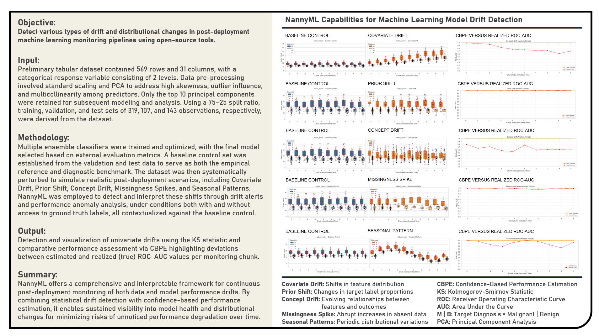
3. References 
- [Book] Reliable Machine Learning by Cathy Chen, Niall Richard Murphy, Kranti Parisa, D. Sculley and Todd Underwood
- [Book] Designing Machine Learning Systems by Chip Huyen
- [Book] Machine Learning Design Patterns by Valliappa Lakshmanan, Sara Robinson and Michael Munn
- [Book] Machine Learning Engineering by Andriy Burkov
- [Book] Engineering MLOps by Emmanuel Raj
- [Book] Introducing MLOps by Mark Treveil, Nicolas Omont, Clément Stenac, Kenji Lefevre, Du Phan, Joachim Zentici, Adrien Lavoillotte, Makoto Miyazaki and Lynn Heidmann
- [Book] Practical MLOps by Noah Gift and Alfredo Deza
- [Book] Data Science on AWS by Chris Fregly and Antje Barth
- [Book] Ensemble Methods for Machine Learning by Gautam Kunapuli
- [Book] Applied Predictive Modeling by Max Kuhn and Kjell Johnson
- [Book] An Introduction to Statistical Learning by Gareth James, Daniela Witten, Trevor Hastie and Rob Tibshirani
- [Book] Ensemble Methods: Foundations and Algorithms by Zhi-Hua Zhou
- [Book] Effective XGBoost: Optimizing, Tuning, Understanding, and Deploying Classification Models (Treading on Python) by Matt Harrison, Edward Krueger, Alex Rook, Ronald Legere and Bojan Tunguz
- [Python Library API] nannyML by NannyML Team
- [Python Library API] NumPy by NumPy Team
- [Python Library API] pandas by Pandas Team
- [Python Library API] seaborn by Seaborn Team
- [Python Library API] matplotlib.pyplot by MatPlotLib Team
- [Python Library API] itertools by Python Team
- [Python Library API] sklearn.experimental by Scikit-Learn Team
- [Python Library API] sklearn.preprocessing by Scikit-Learn Team
- [Python Library API] scipy by SciPy Team
- [Python Library API] sklearn.tree by Scikit-Learn Team
- [Python Library API] sklearn.ensemble by Scikit-Learn Team
- [Python Library API] sklearn.metrics by Scikit-Learn Team
- [Python Library API] xgboost by XGBoost Team
- [Python Library API] lightgbm by LightGBM Team
- [Python Library API] catboost by CatBoost Team
- [Python Library API] StatsModels by StatsModels Team
- [Python Library API] SciPy by SciPy Team
- [Article] Comprehensive Comparison of ML Model Monitoring Tools: Evidently AI, Alibi Detect, NannyML, WhyLabs, and Fiddler AI by Tanish Kandivlikar (Medium)
- [Article] Monitoring AI in Production: Introduction to NannyML by Adnan Karol (Medium)
- [Article] Data Drift Explainability: Interpretable Shift Detection with NannyML by Marco Cerliani (Towards Data Science)
- [Article] An End-to-End ML Model Monitoring Workflow with NannyML in Python by Bex Tuychiyev (DataCamp)
- [Article] Detecting Concept Drift: Impact on Machine Learning Performance by Michal Oleszak (NannyML.Com)
- [Article] Estimating Model Performance Without Labels by Jakub Białek (NannyML.Com)
- [Article] Monitoring Workflow for Machine Learning Systems by Santiago Víquez (NannyML.Com)
- [Article] Don’t Let Yourself Be Fooled by Data Drift by Santiago Víquez (NannyML.Com)
- [Article] Understanding Data Drift: Impact on Machine Learning Model Performance by Jakub Białek (NannyML.Com)
- [Article] NannyML’s Guide to Data Quality and Covariate Shift by Magdalena Kowalczuk (NannyML.Com)
- [Article] From Reactive to Proactive: Shift your ML Monitoring Approach by Qiamo (Luca) Zheng (NannyML.Com)
- [Article] How to Detect Under-Performing Segments in ML Models by Kavita Rana (NannyML.Com)
- [Article] Building Custom Metrics for Predictive Maintenance by Kavita Rana(NannyML.Com)
- [Article] 3 Custom Metrics for Your Forecasting Models by Kavita Rana (NannyML.Com)
- [Article] There's Data Drift, But Does It Matter? by Santiago Víquez (NannyML.Com)
- [Article] Monitoring Custom Metrics without Ground Truth by Kavita Rana (NannyML.Com)
- [Article] Which Multivariate Drift Detection Method Is Right for You: Comparing DRE and DC by Miles Weberman (NannyML.Com)
- [Article] Prevent Failure of Product Defect Detection Models: A Post-Deployment Guide by Kavita Rana (NannyML.Com)
- [Article] Common Pitfalls in Monitoring Default Prediction Models and How to Fix Them by Miles Weberman (NannyML.Com)
- [Article] Why Relying on Training Data for ML Monitoring Can Trick You by Kavita Rana (NannyML.Com)
- [Article] Estimating Model Performance Without Labels by Jakub Białek (NannyML.Com)
- [Article] Using Concept Drift as a Model Retraining Trigger by Taliya Weinstein (NannyML.Com)
- [Article] Retraining is Not All You Need by Miles Weberman (NannyML.Com)
- [Article] A Comprehensive Guide to Univariate Drift Detection Methods by Kavita Rana (NannyML.Com)
- [Article] Stress-free Monitoring of Predictive Maintenance Models by Kavita Rana (NannyML.Com)
- [Article] Effective ML Monitoring: A Hands-on Example by Miles Weberman (NannyML.Com)
- [Article] Don’t Drift Away with Your Data: Monitoring Data Drift from Setup to Cloud by Taliya Weinstein (NannyML.Com)
- [Article] Comparing Multivariate Drift Detection Algorithms on Real-World Data by Kavita Rana (NannyML.Com)
- [Article] Detect Data Drift Using Domain Classifier in Python by Miles Weberman (NannyML.Com)
- [Article] Guide: How to evaluate if NannyML is the right monitoring tool for you by Santiago Víquez (NannyML.Com)
- [Article] How To Monitor ML models with NannyML SageMaker Algorithms by Wiljan Cools (NannyML.Com)
- [Article] Tutorial: Monitoring Missing and Unseen values with NannyML by Santiago Víquez (NannyML.Com)
- [Article] Monitoring Machine Learning Models: A Fundamental Practice for Data Scientists and Machine Learning Engineers by Saurav Pawar (Medium)
- [Article] Failure Is Not an Option: How to Prevent Your ML Model From Degradation by Maciej Balawejder (Medium)
- [Article] Managing Data Drift and Data Distribution Shifts in the MLOps Lifecycle for Machine Learning Models by Abhishek Reddy (Medium)
- [Article] “You Can’t Predict the Errors of Your Model”… Or Can You? by Samuele Mazzanti (Medium)
- [Article] Understanding Concept Drift: A Simple Guide by Vitor Cerqueira (Medium)
- [Article] Detecting Covariate Shift: A Guide to the Multivariate Approach by Michał Oleszak (Medium)
- [Article] Data Drift vs. Concept Drift: Differences and How to Detect and Address Them by DataHeroes Team (DataHeroes.AI)
- [Article] An Introduction to Machine Learning Engineering for Production /MLOps — Concept and Data Drifts by Praatibh Surana (Medium)
- [Article] Concept Drift and Model Decay in Machine Learning by Ashok Chilakapati (Medium)
- [Article] Data Drift: Types of Data Drift by Numal Jayawardena (Medium)
- [Article] Monitoring Machine Learning models by Jacques Verre (Medium)
- [Article] Data drift: It Can Come At You From Anywhere by Tirthajyoti Sarkar (Medium)
- [Article] Drift in Machine Learning by Piotr (Peter) Mardziel (Medium)
- [Article] Understanding Dataset Shift by Matthew Stewart (Medium)
- [Article] Calculating Data Drift in Machine Learning using Python by Vatsal (Medium)
- [Article] 91% of ML Models Degrade in Time by Santiago Víquez (Medium)
- [Article] Model Drift in Machine Learning by Kurtis Pykes (Medium)
- [Article] Production Machine Learning Monitoring: Outliers, Drift, Explainers & Statistical Performance by Alejandro Saucedo (Medium)
- [Article] How to Detect Model Drift in MLOps Monitoring by Amit Paka (Medium)
- [Article] “My data drifted. What’s next?” How to handle ML model drift in production. by Elena Samuylova (Medium)
- [Article] Machine Learning Model Drift by Sophia Yang (Medium)
- [Article] Estimating the Performance of an ML Model in the Absence of Ground Truth by Eryk Lewinson (Medium)
- [Article] Ensemble: Boosting, Bagging, and Stacking Machine Learning by Jason Brownlee (MachineLearningMastery.Com)
- [Article] Stacking Machine Learning: Everything You Need to Know by Ada Parker (MachineLearningPro.Org)
- [Article] Ensemble Learning: Bagging, Boosting and Stacking by Edouard Duchesnay, Tommy Lofstedt and Feki Younes (Duchesnay.GitHub.IO)
- [Article] Stack Machine Learning Models: Get Better Results by Casper Hansen (Developer.IBM.Com)
- [Article] GradientBoosting vs AdaBoost vs XGBoost vs CatBoost vs LightGBM by Geeks for Geeks Team (GeeksForGeeks.Org)
- [Article] A Gentle Introduction to the Gradient Boosting Algorithm for Machine Learning by Jason Brownlee (MachineLearningMastery.Com)
- [Article] The Ultimate Guide to AdaBoost Algorithm | What is AdaBoost Algorithm? by Ashish Kumar (MyGreatLearning.Com)
- [Article] A Gentle Introduction to Ensemble Learning Algorithms by Jason Brownlee (MachineLearningMastery.Com)
- [Article] Ensemble Methods: Elegant Techniques to Produce Improved Machine Learning Results by Necati Demir (Toptal.Com)
- [Article] The Essential Guide to Ensemble Learning by Rohit Kundu (V7Labs.Com)
- [Article] Develop an Intuition for How Ensemble Learning Works by by Jason Brownlee (Machine Learning Mastery)
- [Article] Mastering Ensemble Techniques in Machine Learning: Bagging, Boosting, Bayes Optimal Classifier, and Stacking by Rahul Jain (Medium)
- [Article] Ensemble Learning: Bagging, Boosting, Stacking by Ayşe Kübra Kuyucu (Medium)
- [Article] Ensemble: Boosting, Bagging, and Stacking Machine Learning by Aleyna Şenozan (Medium)
- [Article] Boosting, Stacking, and Bagging for Ensemble Models for Time Series Analysis with Python by Kyle Jones (Medium)
- [Article] Different types of Ensemble Techniques — Bagging, Boosting, Stacking, Voting, Blending by Abhishek Jain (Medium)
- [Article] Mastering Ensemble Techniques in Machine Learning: Bagging, Boosting, Bayes Optimal Classifier, and Stacking by Rahul Jain (Medium)
- [Article] Understanding Ensemble Methods: Bagging, Boosting, and Stacking by Divya bhagat (Medium)
- [Video Tutorial] Concept Drift Detection with NannyML | Webinar by NannyML (YouTube)
- [Video Tutorial] Fooled by Data Drift: How to Monitor ML Without False Positives by NannyML (YouTube)
- [Video Tutorial] Monitoring Custom Metrics Without Access to Targets by NannyML (YouTube)
- [Video Tutorial] Analyzing Your Model's Performance in Production by NannyML (YouTube)
- [Video Tutorial] How to Monitor Predictive Maintenance Models | Webinar Replay by NannyML (YouTube)
- [Video Tutorial] Machine Learning Monitoring Workflow [Webinar] by NannyML (YouTube)
- [Video Tutorial] Monitoring Machine Learning Models on AWS | Webinar by NannyML (YouTube)
- [Video Tutorial] Root Cause Analysis for ML Model Failure by NannyML (YouTube)
- [Video Tutorial] Quantifying the Impact of Data Drift on Machine Learning Model Performance | Webinar by NannyML (YouTube)
- [Video Tutorial] How to Detect Drift and Resolve Issues in Your Machine Learning Models? by NannyML (YouTube)
- [Video Tutorial] Notebooks to Containers: Setting up Continuous (ML) Model Monitoring in Production by NannyML (YouTube)
- [Video Tutorial] Performance Estimation using NannyML | Tutorial in Jupyter Notebook by NannyML (YouTube)
- [Video Tutorial] What Is NannyML? Introducing Our Open Source Python Library by NannyML (YouTube)
- [Video Tutorial] How to Automatically Retrain Your Models with Concept Drift Detection? by NannyML (YouTube)
- [Video Tutorial] How to Use NannyML? Two Modes of Running Our Library by NannyML (YouTube)
- [Video Tutorial] How to Integrate NannyML in Production? | Tutorial by NannyML (YouTube)
- [Video Tutorial] Bringing Your Machine Learning Model to Production | Overview by NannyML (YouTube)
- [Video Tutorial] Notebooks to Containers: Setting Up Continuous (ML) Model Monitoring in Production by NannyML (YouTube)
- [Video Tutorial] ML Performance without Labels: Comparing Performance Estimation Methods (Webinar Replay) by NannyML (YouTube)
- [Course] DataCamp Python Data Analyst Certificate by DataCamp Team (DataCamp)
- [Course] DataCamp Python Associate Data Scientist Certificate by DataCamp Team (DataCamp)
- [Course] DataCamp Python Data Scientist Certificate by DataCamp Team (DataCamp)
- [Course] DataCamp Machine Learning Engineer Certificate by DataCamp Team (DataCamp)
- [Course] DataCamp Machine Learning Scientist Certificate by DataCamp Team (DataCamp)
- [Course] IBM Data Analyst Professional Certificate by IBM Team (Coursera)
- [Course] IBM Data Science Professional Certificate by IBM Team (Coursera)
- [Course] IBM Machine Learning Professional Certificate by IBM Team (Coursera)